Unsteady 2d#
Requirements
This tutorial is designed for advanced modelers and before diving into this tutorial make sure to complete the TELEMAC pre-processing and Telemac2d steady hydrodynamic modeling tutorials.
The case featured in this tutorial was established with the following software:
a text editor, such as Notepad++ (any other text editor will do the job).
Telemac v8p2r0 or newer (standalone installation).
QGIS.
Debian Linux 11 installed on a Virtual Machine (read more in the software chapter).
Get Started#
The steady 2d tutorial hypothesizes that the discharge of a river is constant over time. However, the discharge of a river is never truly constant (i.e., never steady) and varies slightly from second to second, even in controlled rivers. To model the inherently unsteady flows of rivers, we can discretize time-dependent discharge (e.g., a flood hydrograph) in a numerical model as a series of steady discharges. Figure 129 illustrates the discretization of a natural flood hydrograph into steps of steady flows, which will be used in this chapter. Note that the hydrograph starts at Time = 15000, which is the result of the dry-initialized steady2d simulation.
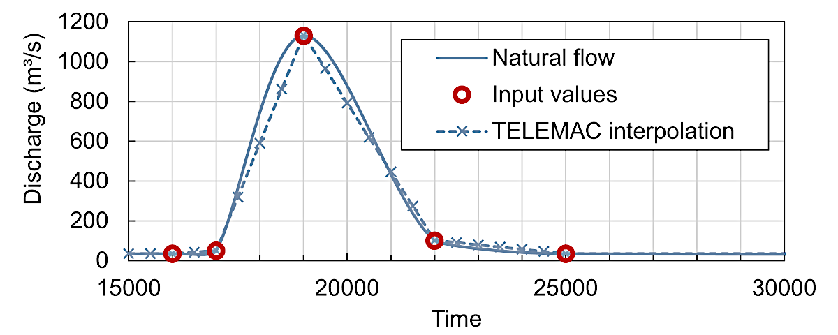
Fig. 129 The discretization of a continuous hydrograph into steps of steady flows (qualitative hydrograph for this tutorial).#
This chapter features the implementation of a quasi-steady discharge hydrograph into a hydrodynamic Telemac2d simulation through the definition of an inflow sequence (red circles in Fig. 129). The tutorial builds on the steady simulation of a discharge of 35 m\(^3\)/s and requires the following data from the pre-processing and steady2d tutorials, which can be downloaded by clicking on the filenames:
The computational mesh qgismesh.slf file (uses EPSG:32633 - ETRS 89 / UTM zone 33N).
The boundary definitions boundaries.cli file.
The results file r2dsteady.slf of the dry initialized steady 2d simulation ending at
t=15000for 35 m\(^3\)/s.
Consider saving the files in a new folder, such as /unsteady2d-tutorial/.
Unsteady simulation file repository
The simulation files used in this tutorial are available at hydro-informatics/telemac.
Model Adaptations#
The implementation of unsteady flows requires the adaptation of keywords and additional keywords (e.g., for linking liquid boundary files) in the steering (.cas) file from the steady2d tutorial (download steady2d.cas).
View the unsteady steering file
To view the integration of the unsteady simulation keywords in the steering file, download unsteady2d.cas.
Hotstart Initial Conditions#
The following descriptions refer to section 4.1.3 in the Telemac2d manual.
To speed up the calculations and provide a well-converging baseline for the quasi-steady calculations, this tutorial re-uses the output of the steady 2d simulation with dry initial conditions (see the Initial Conditions section). This type of model initialization is also called hotstart. To hotstart the simulation, the steady results file r2dsteady.slf needs to be defined as PREVIOUS COMPUTATION FILE:
COMPUTATION CONTINUED : YES
PREVIOUS COMPUTATION FILE : r2dsteady.slf / results of 35 CMS steady simulation
/ INITIAL TIME SET TO ZERO : 0 / avoid restarting at 15000
An INITIAL TIME SET TO ZERO keyword may be defined to reset the time from the previous computation file from 15000 to 0. However, this tutorial does not use this option and continues at timestep 15000.
To avoid ambiguous definitions of initial conditions, deactivate (i.e., delete or comment out lines with a /) the INITIAL CONDITIONS keyword:
/ INITIAL CONDITIONS : 'ZERO DEPTH'
General Parameters#
To simulate the hydrograph shown in Fig. 129, the simulation must run for at least another 15000 time steps (i.e., from t=15000 to t=30000). Since printing out (intermediate) results has a significant effect on computing time, increase the graphic printout timestep to 500 (i.e., decrease the printout frequency compared to 200 used for the steady simulation):
TIME STEP : 1.
NUMBER OF TIME STEPS : 15000
GRAPHIC PRINTOUT PERIOD : 500
LISTING PRINTOUT PERIOD : 500
Open Boundaries#
This section features the implementation of quasi-steady (unsteady) flow conditions at the open liquid boundaries with a time-dependent inflow hydrograph and a downstream stage-discharge relation (recall the rationales behind the choice of boundary types from the pre-processing tutorial).
Boundary conditions and mass balance
The boundary condition settings affect mass balance, which is a crucial criterion for a sound numerical model. Read more in the spotlight chapter on setting up boundary conditions for mass balance.
Define a Quasi-steady Hydrograph
With the dry-initialized model ending at \(t\)=15000, the hydrograph needs to start at 15000, even though the model start will represent time zero of the unsteady simulation. To implement the triangular-shaped hydrograph shown in Fig. 129, create a new file called inflows.liq in the simulation folder. Open the new inflows.liq file in a text editor and add the red-circled points in Fig. 129 as time-dependent flow information at the upstream (1) and downstream (2) open (liquid) boundaries. In this file:
Add a file header starting with
#signs (commented lines ignored by TELEMAC).Implement 2 columns for the time T (\(t\)) and upstream inflow rate Q(1).
Separate the columns with spaces.
The first column must be time
Twith strictly monotonously increasing values and the last time value must be greater than or equal to the last simulation timestep.
How does Telemac count open (liquid) boundaries?
This and more information on the definition of boundaries is provided in the spotlight chapter on boundary conditions.
Thus, the inflows.liq file should look similar to this:
# Inflow hydrograph
#
T	Q(1)
s	m3/s
15000	35
16000	35
17000	50
19000	1130
22000	101
25000	35
99000	35
The original boundaries.cli file describes the downstream boundary with prescribed Q and H (type 5 5 5). However, in the unsteady calculation, Q needs to be free (otherwise, Q(2) needed to be defined in inflows.liq with an additional column) and for this reason, the boundaries.cli file requires some adaptions:
Open the provided boundaries.cli file with a text editor (e.g., NotepadPlusPlus (Text Editor) on Windows).
Use find-and-replace (e.g.,
CTRL+Hkeys in Notepad++, orCTRL+Fkeys in other text editors):Find
5 5 5Replace with
4 5 5Click on Replace all upstream boundary nodes.
Save the file as boundaries-unsteady.cli and close it.
To verify the correct settings download boundaries-unsteady.cli for the unsteady simulation.
In the steering file, adapt the file name for the boundary conditions and add the link to inflows.liq:
BOUNDARY CONDITIONS FILE : boundaries-unsteady.cli
/ ...
LIQUID BOUNDARIES FILE : inflows.liq
Rating Curve (Stage-Discharge Relation) To activate the use of a stage-discharge relation for an open (liquid) boundary, the STAGE-DISCHARGE CURVES keyword needs to be added to the steering file. This keyword requires a list consisting of the following integers:
0is the default that deactivates the usage of a stage-discharge curve.1applies prescribed elevations as a function of calculated flow rate (discharge).2applies prescribed flow rates (discharge) as a function of calculated elevation.
The STAGE-DISCHARGE CURVES keyword is a list that assigns one of the three integers (i.e., either 0, 1, or 2) to the open (liquid) boundaries. In this tutorial, the setting STAGE-DISCHARGE CURVES : 0;1 activates the use of a Stage-discharge relation for the downstream boundary only where the upstream open boundary number 1 is set to 0 and the downstream open boundary number 1 is set to 0.
The form (curve) of the Stage-discharge relation needs to be defined in a stage-discharge file (ASCII text format). Such files typically apply to the downstream boundary of a model at control sections (e.g., a free overflow weir). This tutorial uses the following relationship that is stored in a file called ratingcurve.txt (download):
# Downstream ratingcurve.txt
#
Z(2)	Q(2)
m	m3/s
371.33	35
371.45	50
371.86	101
375.73	1130
379.08	2560
How to assign different stage-discharge curves at multiple boundaries?
To define stage-discharge relations at multiple open boundaries (e.g., at river diversions or tributaries), add the curves to the same file. TELEMAC automatically recognizes where the curves apply by the number given in parentheses after the parameter name in the column header. For instance, in the above example for this tutorial, the column headers Z(2) and Q(2) tell TELEMAC to use these values for the second (i.e., here, the downstream) open boundary. The column order is not important because TELEMAC reads the curve type (i.e., either \(Q(Z)\) or \(Z(Q)\)) from the STAGE-DISCHARGE CURVES keyword.
The following file block would prescribe Stage-discharge relations to the upstream and downstream boundary conditions in this tutorial. However, the file cannot be used here unless the upstream boundary type is changed to 5 5 5 (prescribed H and Q) in the boundaries.cli file (read more in the pre-processing tutorial).
#
# Downstream Rating Curve
#
Z(2)	Q(2)
m	m3/s
371.33	35
371.45	50
371.86	101
375.73	1130
379.08	2560
#
# Upstream Rating Curve
#
Q(1)  Z(1)
m3/s  m
35    371.33
50    371.45
101   371.86
1130  375.73
2560  379.08
To use the stage-discharge file, define the STAGE-DISCHARGE … keywords in the steering file:
/ steering.cas
STAGE-DISCHARGE CURVES : 0;1
STAGE-DISCHARGE CURVES FILE : ratingcurve.txt
Remove Ambiguous Open Boundary Definition Keywords
To avoid ambiguous definitions of the open boundaries conditions, deactivate (i.e., delete or comment out lines with a /) the PRESCRIBED … keywords in the steering file:
/ PRESCRIBED FLOWRATES  : 35.;0.
/ PRESCRIBED ELEVATIONS : 374.80565;371.33
Numerical Parameters#
The predictor-corrector schemes (SCHEME FOR … keywords defined with 3, 4, 5, or 15 rely on a parameter defining the number of iterations at every timestep for convergence (see the steady2d tutorial). For quasi-steady simulations, Telemac developers recommend setting this parameter to 2 or slightly larger (section 7.2.1 in the Telemac2d manual). Therefore, add the following line to the steering file:
NUMBER OF CORRECTIONS OF DISTRIBUTIVE SCHEMES : 2
Control Sections#
A consistent way to verify fluxes at open boundaries or other particular lines (e.g., tributary inflows or diversions) is to use the CONTROL SECTIONS keyword. A control section is defined by a sequence of neighboring node numbers. For instance, to verify the fluxes over the open boundaries in this tutorial, check out the node numbers in the boundaries.cli file (e.g., 144 to 32 for the upstream and 34 to 5 for the downstream boundary). Then, create a new text file (e.g., control-sections.txt) and:
Add one comment line with some short information (e.g.,
# control sections input file). Note that this line is mandatory.In the second line add a space-separated list of 2 integers where
the first integer defines the number of cross-sections, and
the second integer defines if node numbers (i.e., IDs from boundaries.cli or qgismesh.slf) or coordinates will be defined. A negative number enables the node ID-mode, and a positive number enables the coordinates-mode.
Define as many cross sections as defined with the first integer. Every cross-section definition consists of two lines:
The first line is a string (text) without spaces that is naming the cross-section (e.g.,
inflow_cs).The second line consists of two numbers defining the start and end points of the cross-sections. If the second integer in the file line is negative, provide two space-separated integers. If the second integer is positive, provide two space-separated pairs of coordinates (put a space between coordinates).
For example, the following control-sections.txt file can be used with the steady simulation in this tutorial (download control-sections.txt).
# control sections steady2d
2 -1
Inflow_boundary
144 32
Outflow_boundary
34 5
Expand to view an example for coordinate-based control sections
The following control section file uses point coordinates rather than node ID numbers to define three sections. Read more in Gifford-Miears and Leon [GML13] (i.e., section 4.1.2 in the Baxter tutorial).
# control section file using coordinates
3 0
affluent_creek
19572355.895577 626823.06664 1952347.2733 626923.9554
main_river_upstream
1946449.824 635349.6070 194.919 635209.807
main_river_downstream
1967737.56993 620784.415608 1967998.16429 620638.17849
The second line in this file tells TELEMAC to use 2 control sections, which are defined by node IDs (-1). To use the control sections for the simulation add the following to the steering file:
/ steady2d.cas
/ ...
SECTIONS INPUT FILE :  control-sections.txt
SECTIONS OUTPUT FILE : r-control-flows.txt
Thus, re-running the simulation will write the fluxes across the two define control sections to a file called r-control-flows.txt. The Telemac2d manual provides explanations in section 5.2.2.
Run Telemac2d Unsteady#
Go to the configuration folder of the local TELEMAC installation (e.g., ~/telemac/v9.0.0/configs/) and load the environment (e.g., pysource.openmpi.sh - use the same as for compiling TELEMAC).
cd ~/telemac/v9.0.0/configs
source pysource.gfortranHPC.sh
If you are using the Hydro-Informatics (Hyfo) Mint VM
If you are working with the Mint Hyfo VM, load the TELEMAC environment as follows:
cd ~/telemac/v8p2/configs
source pysource.hyfo-dyn.sh
With the TELEMAC environment loaded, change to the directory where the unsteady simulation lives (e.g., /home/telemac/v9.0.0/mysimulations/unsteady2d-tutorial/) and run the *.cas file by calling the telemac2d.py script.
cd ~/telemac/v9.0.0/mysimulations/unsteady2d-tutorial/
telemac2d.py unsteady2d.cas
Speed up
With parallelism enabled (e.g., in the Mint Hyfo Virtual Machine), speed up the calculation by using multiple cores through the --ncsize=N flag. For instance, the following line runs the unsteady simulation on N=2 cores:
telemac2d.py unsteady2d.cas --ncsize=2
A successful computation should end with the following lines (or similar) in Terminal:
[...]
                    *************************************
                    *    END OF MEMORY ORGANIZATION:    *
                    *************************************

CORRECT END OF RUN

ELAPSE TIME :
                            10  MINUTES
                            32  SECONDS
... merging separated result files

... handling result files
       moving: r2dunsteady.slf
       moving: r-control-sections.txt
... deleting working dir

My work is done
Telemac2d will write the files r2dunsteady.slf and r-control-sections.txt. Both results files are also available in the this eBook’s TELEMAC repository to enable accomplishing the post-processing tutorial:
Post-processing#
Open Boundary Flows#
The unsteady simulation intends to model time-variable flows (fluxes) over the upstream and downstream liquid boundaries. The above-defined control sections enable insights into the correct adaptation of the flow at the upstream inflow boundary (prescribed Q through inflows.liq) and the downstream outflow boundary (prescribed H through ratingcurve.txt). Figure 130 shows the modeled flow rates where the Inflow_boundary shows perfect agreement with inflows.liq and the Outflow_boundary reflects the flattening of the discharge curve in the modeled meandering gravel-cobble bed river.
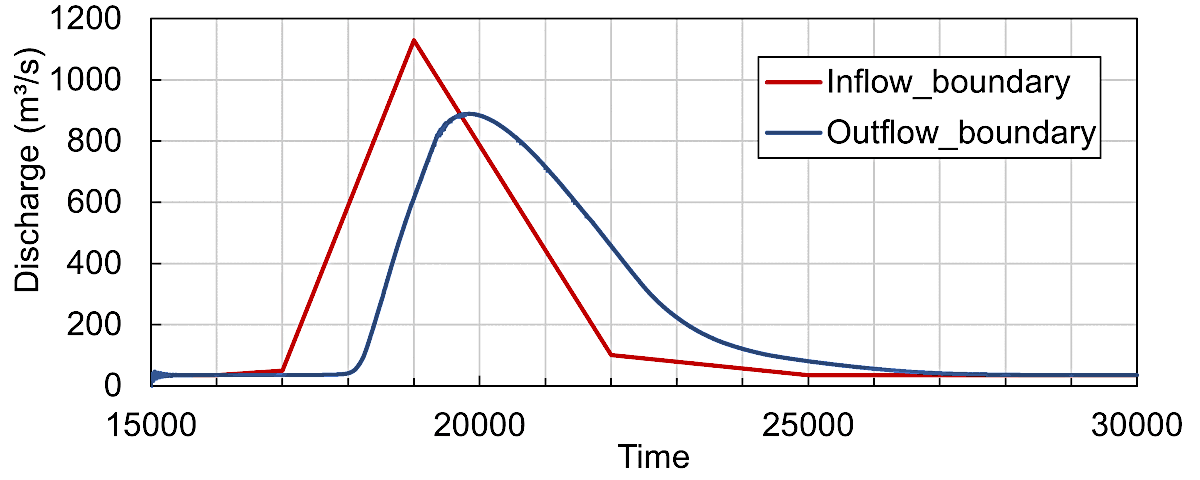
Fig. 130 The simulated flows over the upstream Inflow_boundary and the downstream Outflow_boundary control sections.#
The peak inflow corresponds to the specified 1130 m\(^3\)/s while the outflow peak discharge is only 889 m\(^3\)/s and the peak takes about 1070 seconds (inflow at \(t\)=19000 and outflow at \(t\approx\) 20070) to travel through the section.
Resolve volume balance issues in unsteady simulations
The total inflow and outflow volumes in the here featured simulation amount to 3479930.958 m\(^3\) and 3430100.437 m\(^3\), respectively. Thus, there is a total volume error of 1.4\(%\). To overcome such issues, the Telemac2d manual recommends using a minimum value for water depth to define when a cell is wet or dry. At the same time, the developers do not recommend using a minimum water depth for most simulations and emphasize to use this option only for unsteady (quasi-steady) simulations. Defining a minimum water depth requires setting the TREATMENT OF THE TIDAL FLATS keyword to 2 (read more in the steady2d tutorial), which is neither compatible with parallelization routines, nor with the here used SCHEME FOR ADVECTION ... : 14 settings. Thus, better results but long non-parallelized quasi-steady calculations could be supposedly obtained with the following keywords in the steering file:
OPTION FOR THE TREATMENT OF TIDAL FLATS : 2 / use segment-wise flux control
MINIMUM VALUE OF DEPTH : 0.1 / in meters
Visualization with QGIS#
The results of the unsteady simulation can be visualized and snapshots exported to raster (e.g., GeoTIFF) or shapefile formats in QGIS, similar as explained in the steady2d post-processing. Specifically, the latest QGIS releases enable to load the Selafin results mesh file (here: r2dunsteady.slf) as a QGIS mesh layer. Therefore, launch QGIS, go to the Layer menu and click on Add Layer > Add Mesh Layer…. In the popup window (Data Source Manager / Mesh), select r2dunsteady.slf, click Add, and Close. Figure 131 shows the imported r2dunsteady mesh layer in QGIS with a Softlight blending (set in the Symbology) on google satellite imagery.
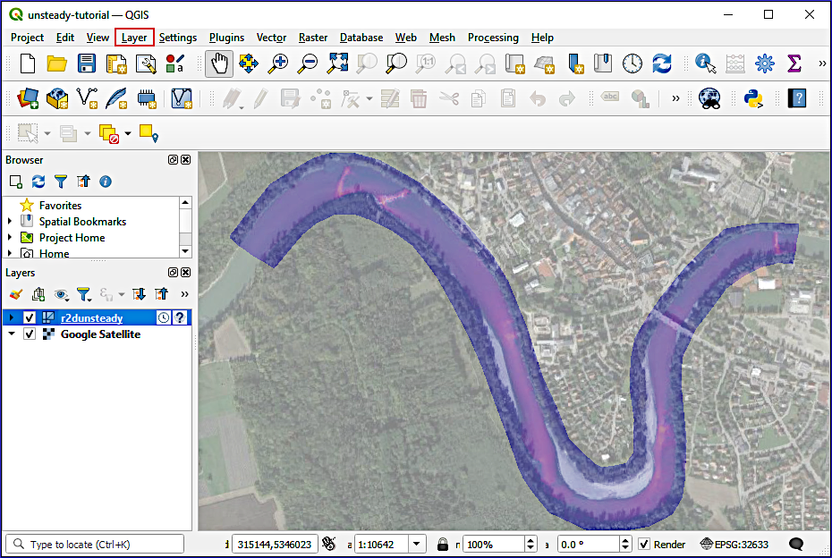
Fig. 131 The unsteady (quasi-steady) simulation results file r2dunsteady.slf imported as mesh layer in QGIS and super-positioned on google satellite imagery [Goond].#
r2dunsteady.slf (results file) not correctly showing in QGIS
Is the results file r2dunsteady.slf not showing up in QGIS? Make sure to import it with its correct georeference: EPSG:32633 (ETRS 89 / UTM zone 33N).
The simulation output parameters (e.g., U, V, or Q) at a selected timestep can be controlled in the layer properties of the r2dunsteady layer (double-click on it in the Layers panel).
To create a video of simulation results, use the Time Controller (see activation in Fig. 132). The frequency of images can be set through clicking on the cogwheel of the time controller, and image sequences played by clicking in the Play button. Additionally, Fig. 126 uses an overlay of water depth pixel colors (contour plot), and flow velocity vectors, defined in the Layer Styling panel. The North and discharge arrows, and the title are Decorators, which can be found in View > Decorators.
Expand to see the Time Controller
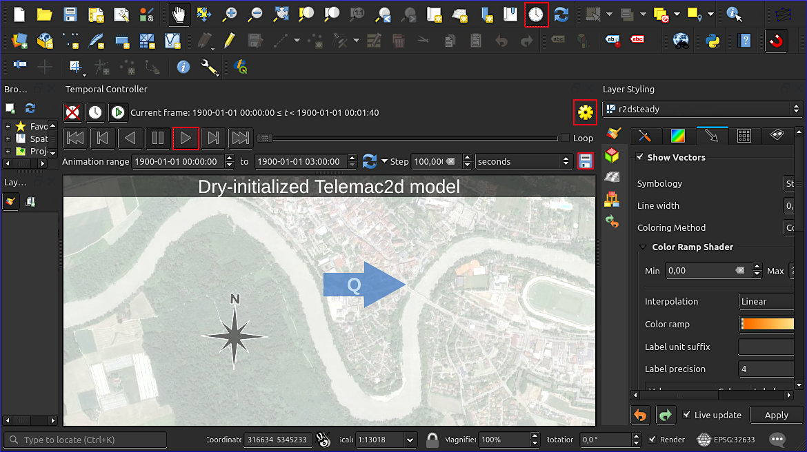
Fig. 132 The activated time controller in QGIS enables to move along the time axis of modeled quantities (background map: Google [Goond] satellite imagery). The red-highlighted buttons activate the time controller, play the sequence of images of selected quantities, provide a setting for playing a frequency of images per second, and enable saving images of all timesteps (see instructions below).#
The exported series of images can be converted to a video with video-editing software, such as the easy and free-to-use OpenShot (good for Windows) or kdenlive (good for Linux) tools. The below-shown box features an exemplary video created with kdenlive.
Expand to view the results as video
Sebastian Schwindt @ Hydro-Morphodynamics channel on YouTube.