Geospatial Data#
Tip
Use QGIS to display geospatial data and to create maps in PDF or image formats (e.g., tif, png, jpg). In addition, the QGIS Tutorial provides an easy and interactive walk through geospatial analyses.
Geodata explained on YouTube
Watch this section as a video on the @Hydro-Morphodynamics channel on YouTube.
Geodata Sources#
Geospatial data can be retrieved for various purposes from different sources. Here are some of them:
Geographical, atlas map-like data are provided by naturalearthdata.com (e.g., with their 227-mb Natural Earth quick start kit).
DEMs, oceanographic and more water-related maps are available at the US’ NOAA Geo-platform and its TDS Catalog
OpenStreetMap data extractions are available at https://download.geofabrik.de/
Satellite imagery is available at
the eesa’s copernicus open access hub (Sentinel-2)
planet.com (commercial)
LiDAR data can be found at opentopography.org.
Climatological data are provided by NASA Earth Observation.
Meteorological (e.g., temperature or precipitation) and real-time satellite data are available at wunderground.com and its wundermap.
Climate and meteorological data and forecasts are available at cds.climate.copernicus.eu, including, for example, ERA5 monthly averaged temperature data
Data on land use (including canopy cover), socioeconomic characteristics, and global change are available at the FAO GeoNetwork or the archived ISCGM Global Map portal (go to their GitHub archive).
Topographical data (1 to 5-m resolution) from the state of Bavaria, Germany, can be found at https://www.ldbv.bayern.de.
Topographical data from EU countries can be found at https://www.mapsforeurope.org.
Visualization#
GIS software is needed to display geospatial data and many tools exist. This website primarily provides examples using QGIS. Since the use of GIS software, especially QGIS, is necessary for several sections in this eBook, explanations on how to install QGIS are already included in the Geospatial Software.
Tip
The QGIS Tutorial features the basics of geospatial data handling with QGIS.
Geodatabase#
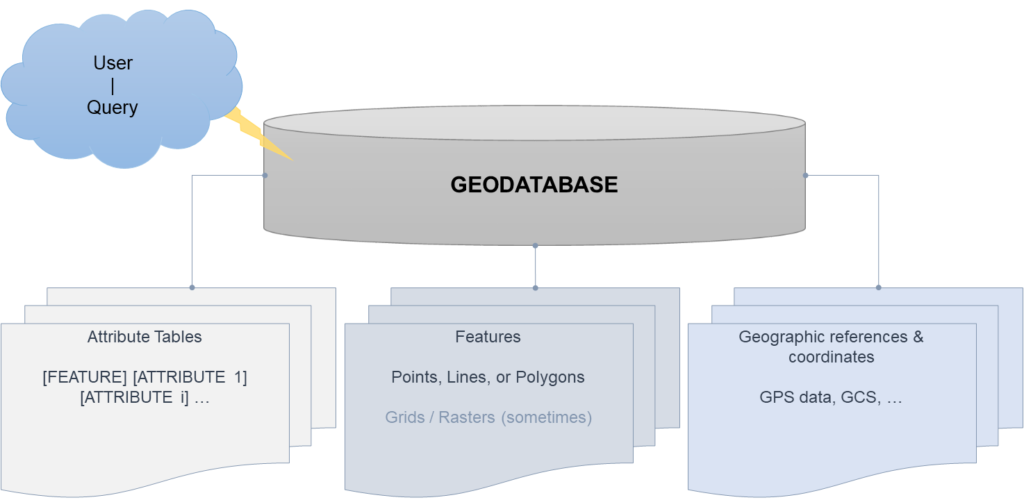
A geodatabase (also known as spatial database) can store, query (e.g., using Structured Query Language SQL), or modify data with geographic references (geospatial data). Primarily, geospatial data consist of vector data (see shapefiles), but raster data can also be implemented. A geodatabase links these data with attribute tables and geographic coordinates. A special feature of geodatabases is that they can be visualized and manipulated via a (web or local) GIS (geographic information system) server. For instance, software like QGIS (or ArcGIS Pro) enables to create maps and make queries on a kind of local server using locally stored geodata. The typical geodatabase format is .gdb, which functions as a directory in QGIS or ArcGIS, and the maximum size of a .gdb file is 1 terabyte.

Fig. 32 The functional skeleton of a geodatabase.#
Vector Data#
Vector data are visually smooth and efficient for overlay operations, especially regarding shape-driven geo-information such as roads or surface delineations. Vector data are characterized as being little storage-intensive, easy to scale, and compatible with relational environments. Common formats are .shp, JSON or TIN.
The shapefile format was invented by Esri (download their whitepaper as PDF) and information contained in a shapefile can be:
Polygons (surface patches),
Points with x-y-z coordinates and an m field containing point data, and
(Poly) lines consisting of lines defined by start points and endpoints.
Shapefile#
Note
The gdal.ogr driver name for shapefile handling is ogr.GetDriverByName('ESRI Shapefile').
A shapefile consists of multiple files on the disk with the following essential parts:
a
.shpfile, where geometries are stored,a
.shxfile, where indices of the geometries are stored,a
.prjfile that stores the projection, anda
.dbffile containing attribute information (constitutes the attribute table).
These files need to be in the same folder - otherwise, the shapefile is incomplete and does not work (correctly). A couple of other files may occur when we manipulate a shapefile (e.g., .atx, .sb*, .shp.xml, .cpg, .mxs, .ai*, or .fb*), but we can ignore those files.
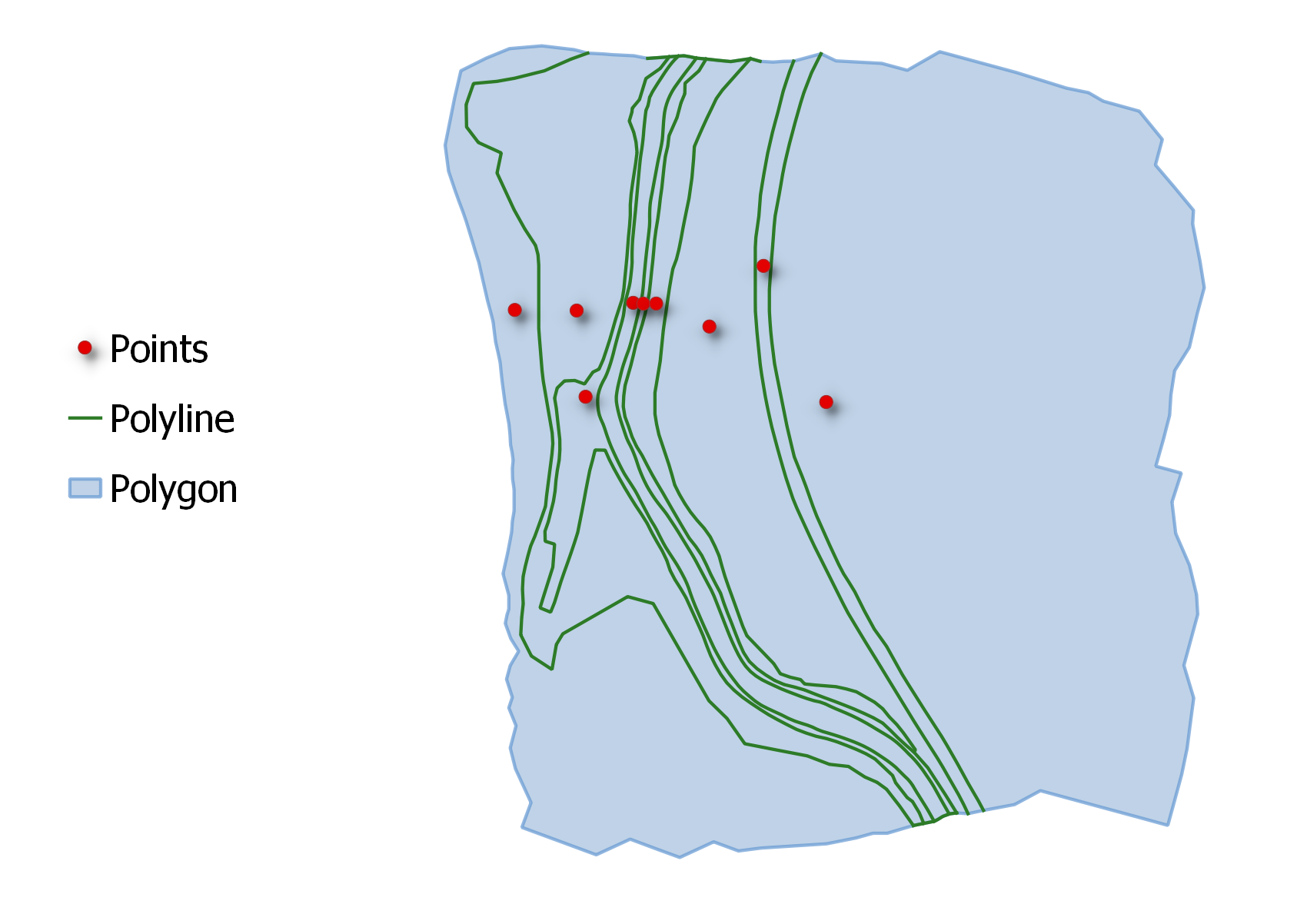
Shapefile vector data typically has an attribute table (just like any other geodatabase) in which every polygon, line, or point object can be assigned an attribute value. Attributes are defined by columns along with their names (column headers) and can have numeric (e.g., float, double, int, or long), text (string), or date/time (e.g. yyyymmdd or HH:MM:SS) formats.

Fig. 33 Illustration of point (red), (poly) line (green), and polygon (blue) shapefile features.#
Shapefile versus Geodatabase#
A shapefile can be understood as a concurring format to a geodatabase. Which file format is better? Strictly speaking, both a geodatabase and a shapefile can perform similar operations, but a shapefile requires more storage space to store similar contents, cannot store combinations of data and time, nor does it support raster files or Null (not-a-number) values. Thus, geodatabases have a technical advantage over shapefiles, but the usage of shapefiles is popular and many geospatial operations focus on shapefile manipulations.
Triangulated Irregular Network (TIN)#
A triangulated irregular network (TIN) represents a surface consisting of multiple triangles. In hydraulic engineering and water resources research, one of the most important usages of TIN is the generation of computational meshes for numerical models read more in the BASEMENT tutorial, for example). In such models, a TIN consists of lines and nodes forming georeferenced, three-dimensionally sloped triangles of the surface, which represent a digital elevation model (DEM). TIN nodes have georeferenced coordinates and potentially more attribute information such as node IDs and elevation. The advantage of a TIN DEM over a raster (see below) DEM is that it requires less storage space. Alas, manipulating a TIN is not that easy like manipulating a raster. The below figure shows an example TIN created with matplotlib.tri.TriAnalyzer, and based on a showcase from the matplotlib docs. The file ending of a TIN is .tin.

Fig. 34 Illustration of a TIN.#
GeoJSON#
Note
The gdal.ogr driver name for shapefile handling is ogr.GetDriverByName('GeoJSON').
GeoJSON is an open format for representing geographic data with simple feature access standards, where JSON denotes JavaScript Object Orientation (read more about JSON file manipulation in the Python basics). The GeoJSON file name ending is .geojson and a file typically has the following structure:
{
  "type": "FeatureCollection",
  "features": [
    {
      "type": "Feature",
      "geometry": {
        "type": "Point",
        "coordinates": [9.104028940200806, 48.74417005744522]
      },
      "properties": {
        "name": "IWS"
      }
    }
  ]
}
While GeoJSON metadata can provide height information (z values) as a properties value, there is a more suitable offspring to encode geospatial topology in the form of the still rather young TopoJSON format. To manipulate GeoJSON files with Python, go to the geojson section. To build a customized GeoJSON file, visit geojson.io
Gridded Cell (Raster) Data#
Raster datasets store pixel values (cells), which require large storage space, but have a simple structure. Another big advantage of rasters is the possibility to perform geospatial algebra and statistical analyses. Common raster dataset formats are, among others, .tif (GeoTIFF), GRID (a folder with BND, HDR, STA, VAT, and other files), .flt (floating points), ASCII (American Standard Code for Information Interchange), and many more image-like file types.
Tip
Preferably use the GeoTIFF format for raster analyses. A GeoTIFF file typically includes a .tif file (with heavy data) and a .tfw (a six-line plain text world file containing georeference information) file.
Note
The gdal driver name for GeoTIFF handling is gdal.GetDriverByName('GTiff').

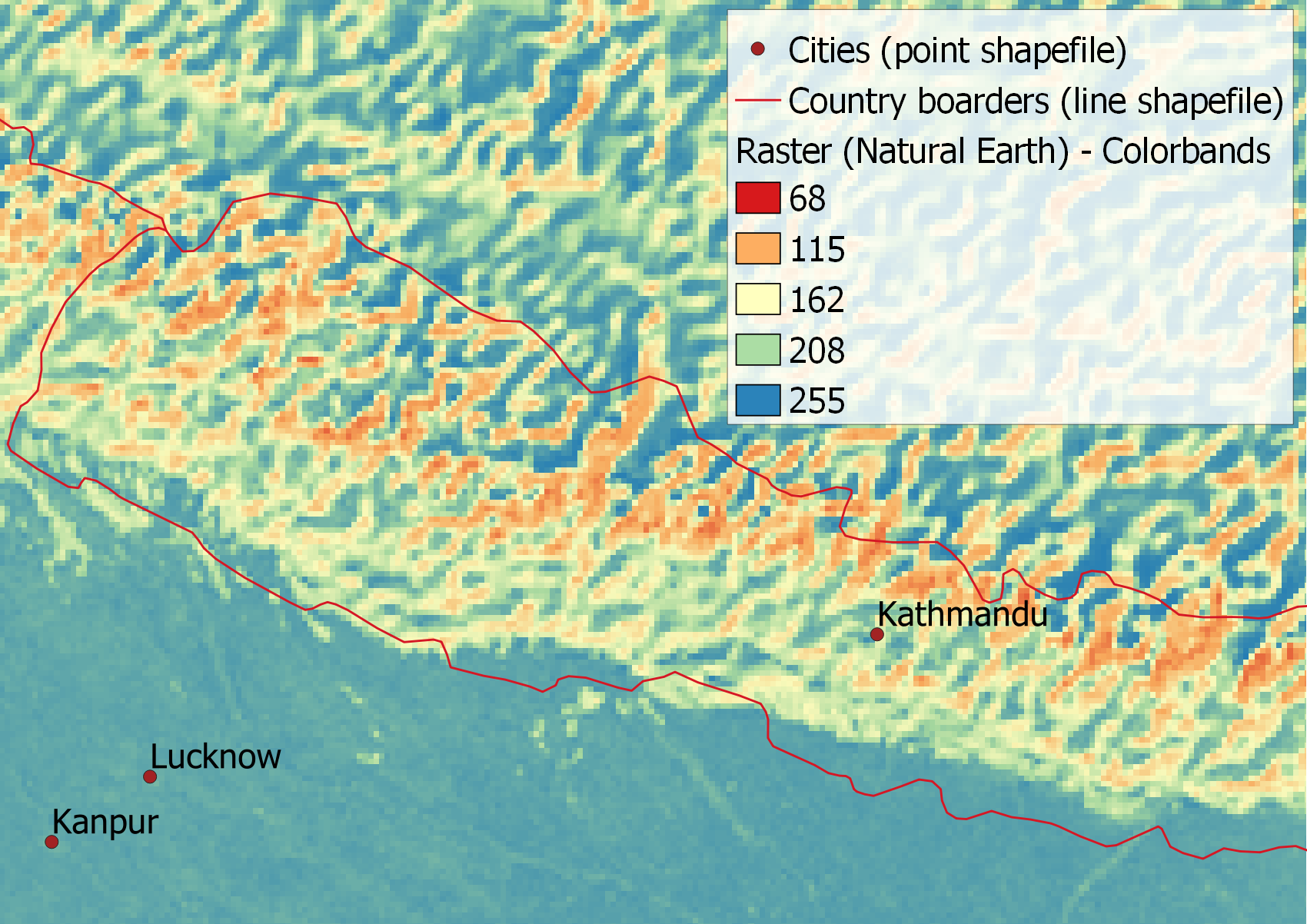
Fig. 35 Illustration of the Natural Earth’s NE1_50M_SR_W.tif raster zoomed on Nepal, with point and line shapefiles indicating major cities and country borders, respectively. Take note of the tile-like appearance of the grid, where every tile corresponds to a 50m-x-50m raster cell.#
Lidar and Underwater Digital Elevation Models (Bathymetries)#
Terrain survey data are often delivered in the shape of an x-y-z point dataset along with point attribute parameters. Three-dimensional datasets of the bare Earth’s topographic surface are referred to as a Digital Elevation Model (read more about DEM terminology in the glossary), which represents the baseline for any physical analysis of a river ecosystem. The underwater topography is called the bathymetry of a river or other water body. Nowadays, x-y-z point clouds for generating a DEM mostly stem from Lidar combined with Echo sounder surveys. Older approaches rely on manual surveying (e.g., with a total station) of cross-sectional river profiles and interpolating the terrain between the profiles. The newer Lidar technique employs light (laser) sources and provides bathymetry data up to 2-m deep water in the form of *.las or the zipped form *.laz files. Deeper waters are mapped with an Echo sounder and the merged Lidar and echo-sounding datasets produce seamless point clouds of river ecosystems, which may be stored in different file types.
Lidar produces massive point clouds, which quickly overcharge even powerful computers. This is why in practice, Lidar data may need to be broken down into smaller zones of less than 106 points each. Particular Lidar processing software (e.g., LAStools) is helpful in this task.
Projections and Coordinate Systems#
In geospatial data analyses, a projection represents an approach to flatten (a part of) the globe. In this flattening process, latitudinal (North/South) and longitudinal (West/East) coordinates of a location on the globe (three-dimensional - 3d) are projected onto the coordinates of a two-dimensional (2d) map. When 3d coordinates are projected onto 2d coordinates, distortions occur and there is a variety of projection systems used in geospatial analyses. In practice, this means that if we use geospatial data files with different projections, a distortion effect propagates in all subsequent calculations. It is crucial to avoid distortion effects by ensuring that the same projections and coordinate systems are applied to all geospatial data used. This starts with the creation of a new geospatial layer (e.g., a point vector shapefile) in QGIS (get installation instructions) and should be used consistently in all program codes. To specify a projection or coordinate system; for instance, in QGIS (tutorial in the next section), click on Project > Properties > CRS tab and select a COORDINATE_SYSTEM. For example, an appropriate coordinate system for central Europe is ESRI:31493 (read more in the QGIS docs). Projected systems may vary with regions (local coordinate systems), which can, for example, be found at epsg.io or spatialreference.org.
In shapefiles, information about the projection is stored in a .prj file (recall definitions in the shapefile section), which is a plain text file. The Open Spatial Consortium (OGC) and Esri use Well-Known Text (WKT) files for standard descriptions of coordinate systems and a WKT-formatted .prj file is shown in the code block below. The units and measures defined in the WKT-formatted .prj file also determine the units of WKB (Well-Known Binary) definitions of geometries such as line length (e.g., in meters, feet, or many more), or polygon area (square meters, square kilometers, acres, and many more).
PROJCS["unknown",GEOGCS["GCS_unknown",
                        DATUM["D_Unknown_based_on_GRS80_ellipsoid",SPHEROID["GRS_1980",6378137.0,298.257222101]],
                        PRIMEM["Greenwich",0.0],UNIT["Degree",0.0174532925199433]],
       PROJECTION["Lambert_Conformal_Conic"], PARAMETER["False_Easting",6561666.66666667],
       ..., UNIT["US survey foot",0.304800609601219]]
In GeoJSON files, the standard coordinate system is WGS84 according to the developer’s specifications.
Use EPSG:3857
To ensure that all geometries are measured in meters and powers of meters, use EPSG:3857 (former 900913 - g00glE) to define the WKT-formatted projection file.