Raster (Grid) Handling#
This section introduces geospatial analysis of raster (gridded) data with gdal and rasterstats. For interactive reading and executing code blocks ![]() and find geo02-raster.ipynb, or install Python and JupyterLab locally.
and find geo02-raster.ipynb, or install Python and JupyterLab locally.
Requirements
Make sure to understand gridded raster data, in particular, the
.tif(GeoTIFF) formatAccomplish the QGIS tutorial
Get started
While OSGeo’s
ogrmodule is useful for shapefile handling, raster data are best handled bygdal.Download sample raster datasets from River Architect. In particular, this section uses GeoTIFF raster data located in
RiverArchitect/SampleData/01_Conditions/2100_sample/.The functions featured in this section are introduced are partially also implemented in flusstools. To use those functions, make sure flusstools is installed and import it as follows:
from flusstools import geotools. Some of the functions shown in this tutorial can then be used withgeotools.function_name().
Watch this section and the Python tutorials in video formats
Watch this section as a video on the @Hydro-Morphodynamics channel on YouTube.
Load raster#
Open Existing Raster Data#
Raster data can be opened in Python code as an instance of gdal.Open("FILENAME"). The following code block provides a function to open any raster specified with the file_name input argument. One of the most important elements when dealing with raster data is the raster band, which takes on a similar data carrier role as GetLayer in shapefile handling. To access the raster band, the below-shown open_raster function:
Enables error and warning feedback with
gdal.UseExceptions()(this step is vital when using gdal).Opens the provided raster
file_nameembraced bytry-exceptstatements to inform if and why a potential error occurred while opening the raster.Opens the raster band number stated in the optional
band_numberkeyword argument withraster_band = raster.GetRasterBand(band_number)(the default value is1).Returns the raster and raster band objects.
from osgeo import gdal


def open_raster(file_name, band_number=1):
    """
    Open a raster file and access its bands
    :param file_name: STR of a raster file directory and name
    :param band_number: INT of the raster band number to open (default: 1)
    :output: osgeo.gdal.Dataset, osgeo.gdal.Band objects
    """
    gdal.UseExceptions()
    # open raster file or return None if not accessible
    try:
        raster = gdal.Open(file_name)
    except RuntimeError as e:
        print("ERROR: Cannot open raster.")
        print(e)
        return None
    # open raster band or return None if corrupted
    try:
        raster_band = raster.GetRasterBand(band_number)
    except RuntimeError as e:
        print("ERROR: Cannot access raster band.")
        print(e)
        return None
    return raster, raster_band
Tip
This function is available in flusstools. For instance, use it with from flusstools import geotools and geotools.open_raster("path/to/raster.tif").
To use the open_raster function, call it with a file name as shown in the following code block with the h001000.tif raster from the River Architect sample data. The script immediately closes the raster again by overwriting the variable with a None-instance to avoid the GeoTIFF file being locked afterward.
import os
file_name = r"" + os.getcwd() + "/geodata/rasters/h001000.tif"
src, depth = open_raster(file_name)
print(src)
print(depth)
depth = None
<osgeo.gdal.Dataset; proxy of <Swig Object of type 'GDALDatasetShadow *' at 0x000001D5E1E95330> >
<osgeo.gdal.Band; proxy of <Swig Object of type 'GDALRasterBandShadow *' at 0x000001D5E1E95300> >
Raster Band Statistics and Toolbox Scripts#
Once the raster and its band are loaded with the above open_raster function, we can access statistical information (e.g., the minimum or the maximum), identify the no-data value (i.e., a pre-defined value that is assigned to pixels without value), or the type of units used.
Python scripts for processing geospatial data can also be embedded as plugins in GIS desktop applications (e.g., as plugins in QGIS or Toolbox in ArcGIS Pro). To run a Python script in a GIS desktop application, it should be written as a standalone script that can receive input arguments. The interested reader can learn more about implementing plugins in QGIS in the QGIS docs.
Note
QGIS wraps many external algorithm types, which are available through the QGIS Processing Toolbox. These algorithms belong, for example, to SAGA or GRASS GIS.
Here we will only write the next code block so that it can be run in a console/terminal application as a standalone script (recall the instructions for writing standalone script).
# make sure to use exceptions
gdal.UseExceptions()

def how2use():
    # provide usage instructions for the script
    print("""
    $ raster_band_info.py [ band number ] input-raster
    """)
    # exit program if wrong input arguments provided
    sys.exit(1)


def get_color_bands(raster_band):
    """
    :param raster_band: osgeo.gdal.Band object
    :output: list of color bands used in raster_band
    """

    # get ColorTable and return False if None
    color_table = raster_band.GetColorTable()
    if color_table is None:
        print("Band has no ColorTable.")
        return None
    else:
        print("Found %i color definitions." % int(color_table.GetCount()))

    # iterate through color_table and append objects found to colors_bands list
    color_bands = []
    for c in range(0, color_table.GetCount() ):
        entry = color_table.GetColorEntry(c)
        if not entry:
            continue
        color_bands.append(str(color_table.GetColorEntryAsRGB(c, entry)))
    return color_bands

def main(band_number, input_file):
    src, band = open_raster(input_file)
    print("Band minimum: ", band.GetMinimum())
    print("Band maximum: ", band.GetMaximum())
    print("No-data value: ", band.GetNoDataValue())
    print("Band unit type: ", band.GetUnitType())

    try:
        print(", ".join(get_color_bands(band)))
    except TypeError:
        print("ColorTable: None")

if __name__ == '__main__':
    # make standalone
    if len( sys.argv ) < 3:
        print("""
        ERROR: Provide two arguments:
        1) the band number (int) and 2) input raster directory (str)
        """)
        how2use()

    main(int(sys.argv[1]), str(sys.argv[2]))
To run this script, save it as raster_band_info.py (e.g., in C:\temp in Windows or ~/temp/ in Linux) and navigate to the script directory in a terminal interface (e.g., in PyCharm’s Terminal, Anaconda Prompt, or the Linux Terminal) using the cd command. Then run the script to get statistics of the water depth raster h001000.tif with (in Windows):
C:\temp\ python raster_band_info.py 1 "C:\temp\geodata\rasters\h001000.tif"
On Linux and with the vflussenv activated tap, for example:
python raster_band_info.py 1 "~/temp/geodata/rasters/h001000.tif"
Band minimum:  0.0
Band maximum:  7.0613012313843
No-data value:  -3.4028234663852886e+38
Band unit type:
Band has no ColorTable.
ColorTable: None
Create and Save a Raster (from Array)#
Raster Drivers#
Just like for shapefile files, the appropriate gdal driver (analogous to ogr drivers) must be loaded to save a raster. To get a full list of gdal raster drivers run:
driver_list = [str(gdal.GetDriver(i).GetDescription()) for i in range(gdal.GetDriverCount())]
driver_list.sort()
print(", ".join(driver_list[:]))
AAIGrid, ACE2, ADRG, AIG, ARCGEN, ARG, AVCBin, AVCE00, AeronavFAA, AirSAR, AmigoCloud, BAG, BIGGIF, BLX, BMP, BNA, BSB, BT, BYN, CAD, CALS, CEOS, COASP, COSAR, CPG, CSV, CSW, CTG, CTable2, Carto, Cloudant, CouchDB, DAAS, DB2ODBC, DERIVED, DGN, DIMAP, DIPEx, DOQ1, DOQ2, DTED, DXF, E00GRID, ECRGTOC, EDIGEO, EEDA, EEDAI, EHdr, EIR, ELAS, ENVI, ERS, ESAT, ESRI Shapefile, ESRIJSON, ElasticSearch, FAST, FIT, FITS, FujiBAS, GFF, GFT, GIF, GML, GMLAS, GMT, GNMDatabase, GNMFile, GPKG, GPSBabel, GPSTrackMaker, GPX, GRASSASCIIGrid, GRIB, GS7BG, GSAG, GSBG, GSC, GTX, GTiff, GXF, GenBin, GeoJSON, GeoJSONSeq, GeoRSS, Geoconcept, Geomedia, HDF4, HDF4Image, HDF5, HDF5Image, HF2, HFA, HTF, HTTP, IDA, IGNFHeightASCIIGrid, ILWIS, INGR, IRIS, ISCE, ISIS2, ISIS3, Idrisi, JAXAPALSAR, JDEM, JML, JP2OpenJPEG, JPEG, KEA, KML, KMLSUPEROVERLAY, KRO, L1B, LAN, LCP, LOSLAS, Leveller, MAP, MBTiles, MEM, MFF, MFF2, MRF, MSGN, MSSQLSpatial, MVT, MapInfo File, Memory, NAS, NDF, NGSGEOID, NGW, NITF, NTv1, NTv2, NWT_GRC, NWT_GRD, ODBC, ODS, OGR_GMT, OGR_PDS, OGR_SDTS, OGR_VRT, OSM, OZI, OpenAir, OpenFileGDB, PAux, PCIDSK, PCRaster, PDF, PDS, PDS4, PGDUMP, PGeo, PLMOSAIC, PLSCENES, PNG, PNM, PRF, PostGISRaster, PostgreSQL, R, RDA, REC, RIK, RMF, ROI_PAC, RPFTOC, RRASTER, RS2, RST, Rasterlite, S57, SAFE, SAGA, SAR_CEOS, SDTS, SEGUKOOA, SEGY, SENTINEL2, SGI, SIGDEM, SNODAS, SQLite, SRP, SRTMHGT, SUA, SVG, SXF, Selafin, TIGER, TIL, TSX, Terragen, TileDB, TopoJSON, UK .NTF, USGSDEM, VDV, VFK, VICAR, VRT, WAsP, WCS, WEBP, WFS, WFS3, WMS, WMTS, Walk, XLS, XLSX, XPM, XPlane, XYZ, ZMap, netCDF
Raster Data Types#
The output raster pixels can be one of the following data types (source: gdal.org/doxygen/):
GDT_UnknownUnknown or unspecified typeGDT_Byte8 bit unsigned integerGDT_UInt1616 bit unsigned integerGDT_Int1616 bit signed integerGDT_UInt3232 bit unsigned integerGDT_Int3232 bit signed integerGDT_Float3232 bit floating pointGDT_Float6464 bit floating pointGDT_CInt16Complex Int16GDT_CInt32Complex Int32GDT_CFloat32Complex Float32GDT_CFloat64Complex Float64
Create a Raster (Array to Raster)#
Knowing the basics of raster handling, data types, and Python, we can create a raster from a numeric array. Since a raster is basically a georeferenced array, it is convenient to convert a numpy array into a raster (band). The function blocks feature the conversion of a numpy array into a GeoTIFF raster according to the following workflow:
Check out the GeoTIFF driver (
driver = gdal.GetDriverByName('GTiff')).Retrieve the array size and (number of rows
rowsand columnscols).Create a new GeoTIFF raster (
new_raster = driver.Create(file_name, cols, rows, 1, eType=rdtype)), wherefile_nameis the directory and name of the new raster file ending on.tif(e.g.,"C:\\temp\\rasters\\new.tif").cols,rowsrepresent the array shape, andeTypeis the geospatial data type (see above list)
Set the geographic origin, which is stored in the
origin(tuple) parameter and defines thepixel_widthandpixel_height(pixel units defined withsrs- see below).Replace
np.nanvalues in the numpy array withnan_value.Instantiate a
bandobject, set theNoDataValuetonan_value, and write the array to theband.Create a spatial reference system object (
srs) as a function of theepsginput parameter and export it to WKT format.Release the raster (flush from cache).
Note
The units defined with the epsg number drive the pixel size, where pixel_width and pixel_height are multipliers of that unit. In the case of epsg=3857, the unit is meters and pixel_width=10 combined with pixel_height=20 creates 10-m wide and 20-m high pixels. In the case of epsg=4326, the unit is (geographic) degrees and 1 degree by 1-degree pixels can have the size of a count®y.
from osgeo import osr


def create_raster(file_name, raster_array, origin=None, epsg=4326, pixel_width=10, pixel_height=10,
                  nan_value=-9999.0, rdtype=gdal.GDT_Float32, geo_info=False):
    """
    Convert a numpy.array to a GeoTIFF raster with the following parameters
    :param file_name: STR of target file name, including directory; must end on ".tif"
    :param raster_array: np.array of values to rasterize
    :param origin: TUPLE of (x, y) origin coordinates
    :param epsg: INT of EPSG:XXXX projection to use - default=4326
    :param pixel_height: INT of pixel height (multiple of unit defined with the EPSG number) - default=10m
    :param pixel_width: INT of pixel width (multiple of unit defined with the EPSG number) - default=10m
    :param nan_value: INT/FLOAT no-data value to be used in the raster (replaces non-numeric and np.nan in array)
                        default=-9999.0
    :param rdtype: gdal.GDALDataType raster data type - default=gdal.GDT_Float32 (32 bit floating point)
    :param geo_info: TUPLE defining a gdal.DataSet.GetGeoTransform object (supersedes origin, pixel_width, pixel_height)
                        default=False
    """
    # check out driver
    driver = gdal.GetDriverByName('GTiff')

    # create raster dataset with number of cols and rows of the input array
    cols = raster_array.shape[1]
    rows = raster_array.shape[0]
    new_raster = driver.Create(file_name, cols, rows, 1, eType=rdtype)

    # apply geo-origin and pixel dimensions
    if not geo_info:
        origin_x = origin[0]
        origin_y = origin[1]
        new_raster.SetGeoTransform((origin_x, pixel_width, 0, origin_y, 0, pixel_height))
    else:
        new_raster.SetGeoTransform(geo_info)

    # replace np.nan values
    raster_array[np.isnan(raster_array)] = nan_value

    # retrieve band number 1
    band = new_raster.GetRasterBand(1)
    band.SetNoDataValue(nan_value)
    band.WriteArray(raster_array)
    band.SetScale(1.0)

    # create projection and assign to raster
    srs = osr.SpatialReference()
    srs.ImportFromEPSG(epsg)
    new_raster.SetProjection(srs.ExportToWkt())

    # release raster band
    band.FlushCache()
To call the function for writing a random numpy array, we can now use the create_raster() function (also available from geotools.create_raster()):
# set the name of the output GeoTIFF raster
raster_name = r"" + os.getcwd() + "/geodata/rasters/random_unis_dem.tif"
# create a random numpy array (DEM-like values) - can be replaced with any other numpy.array
unis_dem = np.random.rand(300, 300) + 455.0
# overwrite one pixel with np.nan
unis_dem[5, 7] = np.nan
# define a raster origin in EPSG:3857
raster_origin = (1013428.396233, 6231555.006177)
# call create_raster to create a 1-m-resolution raster in EPSG:4326 projection
create_raster(raster_name, unis_dem, raster_origin,  pixel_width=1,  pixel_height=1, epsg=3857)
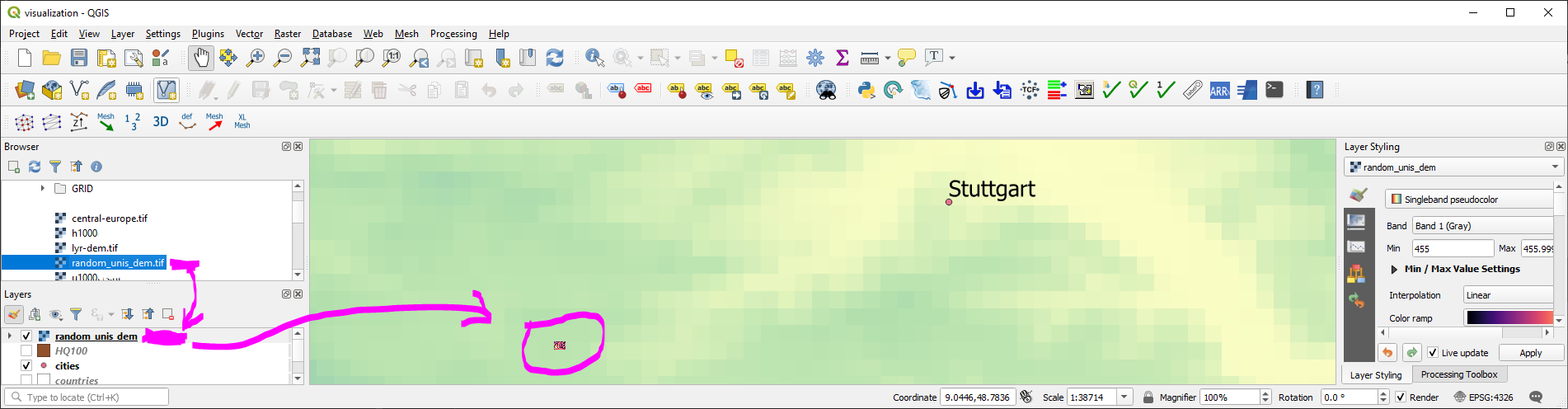
Fig. 49 The new raster containing a random unis_dem point height.#
Raster Calculus (Raster / Band to Array)#
The procedure described with the create_raster() function can be used vice-versa, to create numpy array from raster bands. The raster converted to a numpy array enables algebraic or other logical operations to be applied to existing raster data.
Need an example? In the RiverArchitect SampleData, the units of the water depth raster h001000.tif are in U.S. customary feet and the units of the flow velocity raster u001000.tif are in feet per second. However, to calculate the Froude number (involves the gravity constant) for every pixel based on the two rasters (water depth and flow velocity), it is convenient to convert both rasters into m and m/s, respectively. For this purpose, the following code block features another re-usable, custom function that loads a raster as an array and overwrites NoDataValues with np.nan (raster and band can be instantiated with the above open_raster function):
def raster2array(file_name, band_number=1):
    """
    :param file_name: STR of target file name, including directory; must end on ".tif"
    :param band_number: INT of the raster band number to open (default: 1)
    :output: (1) ndarray() of the indicated raster band, where no-data values are replaced with np.nan
             (2) the GeoTransformation used in the original raster
    """
    # open the raster and band (see above)
    raster, band = open_raster(file_name, band_number=band_number)
    # read array data from band
    band_array = band.ReadAsArray()
    # overwrite NoDataValues with np.nan
    band_array = np.where(band_array == band.GetNoDataValue(), np.nan, band_array)
    # return the array and GeoTransformation used in the original raster
    return raster, band_array, raster.GetGeoTransform()
The raster2array() function is also included in flusstools: geotools.raster2array()
Challenge
The raster2array function returns a tuple, where output[0] corresponds to the array and output[1] is the geo-transformation. Can you optimize the way how this information is returned?
Finally, to create a Froude number GeoTIFF raster, the following code block makes use of the raster2array function for converting the water depth and flow velocity GeoTIFF rasters into a numpy array, performing simple algebraic calculations to convert the rasters to m and m/s, respectively, and save the resulting GeoTIFF file. In detail, the workflow involves to:
Define the input raster file names with directories (
h_fileandu_file),Load original rasters as
ndarraywith theraster2array()function and get the originalGeoTransformdescription,Convert all values from U.S. customary feet to S.I. metric units (recall the feet_to_meter() function from the Python basics), and
Save a new copy of the raster.
h_file = r"" + os.getcwd() + "/geodata/rasters/h001000.tif"
u_file = r"" + os.getcwd() + "/geodata/rasters/u001000.tif"

# load both rasters as arrays
h_ras, h, h_geo_info = raster2array(h_file)
u_ras, u, u_geo_info = raster2array(u_file)

#convert to metric system
h *= 0.3048
u *= 0.3048

# calculate the Froude number as array and avoid zero-division warning messages
with np.errstate(divide="ignore", invalid="ignore"):
    Froude = u / np.sqrt(h * 9.81)

# create Froude raster from array
create_raster(file_name= r"" + os.path.abspath("") + "/geodata/rasters/Fr1000cfs.tif",
              raster_array=Froude, epsg=6418, geo_info=h_geo_info)
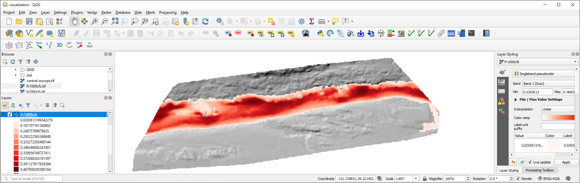
Fig. 50 The Froude number raster calculated with flow velocity and water depth rasters.#
Reproject a Raster#
The transformation (and reprojection) of a raster into another coordinate system involves rotating, shifting, and shearing pixels. If one of these operations is skipped, the reprojected raster may be squeezed, twisted, or placed anywhere in the world but not where it should be placed. Therefore, the approach for the reprojection of a raster into another coordinate reference system implies the following steps:
Retrieve the source and target spatial reference systems (e.g., derive from a
gdal.Datasetor anEPSGauthority code).Read the geo transformation of the source dataset (
gdal.Dataset.GetGeoTransform()).Derive the number of pixels and the spacing between pixels in the new (reprojected) dataset.
Instantiate the new (reprojected) dataset.
Project an image of the source dataset onto the new (reprojected) dataset (
gdal.ReprojectImage()).
The spatial reference system can be derived from a dataset with the explanations in the shapefile section by writing a get_srs() function. The following code block shows the get_srs() function (uses the osr library from osgeo / gdal ), which is also integrated in flusstools (geotools.get_srs()).
def get_srs(dataset):
    """
    Get the spatial reference of any gdal.Dataset
    :param dataset: osgeo.gdal.Dataset (raster)
    :output: osr.SpatialReference
    """
    sr = osr.SpatialReference()
    sr.ImportFromWkt(dataset.GetProjection())
    # auto-detect epsg
    auto_detect = sr.AutoIdentifyEPSG()
    if auto_detect != 0:
        sr = sr.FindMatches()[0][0]  # Find matches returns list of tuple of SpatialReferences
        sr.AutoIdentifyEPSG()
    # assign input SpatialReference
    sr.ImportFromEPSG(int(sr.GetAuthorityCode(None)))
    return sr
ith the open_raster() and get_srs() functions, we have all necessary ingredients to accomplish the raster reprojection workflow in another funcation called reproject_raster(). An additional feature of the function is that it ensures the correct use of osr.CoordinateTransformation, which behaves differently under gdal 3.0 compared with older gdal versions (read more on OSGeo’s GitHub page).
def reproject_raster(source_dataset, source_srs, target_srs):
    """
    Reproject a raster dataset (preferably use through reproject function)
    :param source_dataset: osgeo.ogr.DataSource (instantiate with ogr.Open(SHP-FILE))
    :param source_srs: osgeo.osr.SpatialReference (instantiate with get_srs(source_dataset))
    :param target_srs: osgeo.osr.SpatialReference (instantiate with get_srs(DATASET-WITH-TARGET-PROJECTION))
    """
    # READ THE SOURCE GEO TRANSFORMATION (ORIGIN_X, PIXEL_WIDTH, 0, ORIGIN_Y, 0, PIXEL_HEIGHT)
    src_geo_transform = source_dataset.GetGeoTransform()

    # DERIVE PIXEL AND RASTER SIZE
    pixel_width = src_geo_transform[1]
    x_size = source_dataset.RasterXSize
    y_size = source_dataset.RasterYSize

    # ensure that TransformPoint (later) uses (x, y) instead of (y, x) with gdal version >= 3.0
    source_srs.SetAxisMappingStrategy(osr.OAMS_TRADITIONAL_GIS_ORDER)
    target_srs.SetAxisMappingStrategy(osr.OAMS_TRADITIONAL_GIS_ORDER)

    # get CoordinateTransformation
    coord_trans = osr.CoordinateTransformation(source_srs, target_srs)

    # get boundaries of reprojected (new) dataset
    (org_x, org_y, org_z) = coord_trans.TransformPoint(src_geo_transform[0], src_geo_transform[3])
    (max_x, min_y, new_z) = coord_trans.TransformPoint(src_geo_transform[0] + src_geo_transform[1] * x_size,
                                                       src_geo_transform[3] + src_geo_transform[5] * y_size,)

    # INSTANTIATE NEW (REPROJECTED) IN-MEMORY DATASET AS A FUNCTION OF THE RASTER SIZE
    mem_driver = gdal.GetDriverByName('MEM')
    tar_dataset = mem_driver.Create("",
                                    int((max_x - org_x) / pixel_width),
                                    int((org_y - min_y) / pixel_width),
                                    1, gdal.GDT_Float32)
    # create new GeoTransformation
    new_geo_transformation = (org_x, pixel_width, src_geo_transform[2],
                              org_y, src_geo_transform[4], -pixel_width)

    # assign the new GeoTransformation to the target dataset
    tar_dataset.SetGeoTransform(new_geo_transformation)
    tar_dataset.SetProjection(target_srs.ExportToWkt())

    # PROJECT THE SOURCE RASTER ONTO THE NEW REPROJECTED RASTER
    rep = gdal.ReprojectImage(source_dataset, tar_dataset,
                              source_srs.ExportToWkt(), target_srs.ExportToWkt(),
                              gdal.GRA_Bilinear)
    return tar_dataset
Using the reproject_raster() function in a Python script requires a source dataset and another (orientation) dataset with the new coordinate system into which the source dataset will be projected. The following example shows how to re-project the above-created Froude-number raster into the EPSG=3857 coordinate system for viewing it in QGIS on a Google Satellite basemap (recall basemaps in QGIS tutorial). As orientation data set, use web_frame.tif, which was created on the Google Satellite basemap.
With the get_srs() function that automatically detects the raster projection and spatial reference system, we can use the create_raster() function to reproject the above-created Fr1000cfs.tif raster (e.g., to epsg=4326).
# load original and orientation rasters
source_file_name = r"" + os.path.abspath("") + "/geodata/rasters/Fr1000cfs.tif"
orientation_file_name = r"" + os.path.abspath("") + "/geodata/rasters/web_frame.tif"

src_dataset, src_band = open_raster(source_file_name)
ort_dataset, ort_band = open_raster(orientation_file_name)

src_srs = get_srs(src_dataset)
new_srs = get_srs(ort_dataset)

print("Source EPSG: " + str(src_srs.GetAuthorityCode(None)))
print("Target EPSG: " + str(new_srs.GetAuthorityCode(None)))

# flush orientation dataset
ort_dataset, ort_band = None, None

# create re-projected raster and save as GeoTIFF
reproj_dataset = reproject_raster(src_dataset, src_srs, new_srs)
reproj_file_name = r"" + os.path.abspath("") + "/geodata/rasters/Fr1000cfs_reproj.tif"
array_data = reproj_dataset.ReadAsArray()
new_epsg = int(new_srs.GetAuthorityCode(None))
geo_transformation = reproj_dataset.GetGeoTransform()
create_raster(reproj_file_name, raster_array=array_data, epsg=new_epsg, geo_info=geo_transformation)
reproj_dataset = None
Source EPSG: 6418
Target EPSG: 3857
Plotted in QGIS, the reprojected Froude-number raster looks like this:
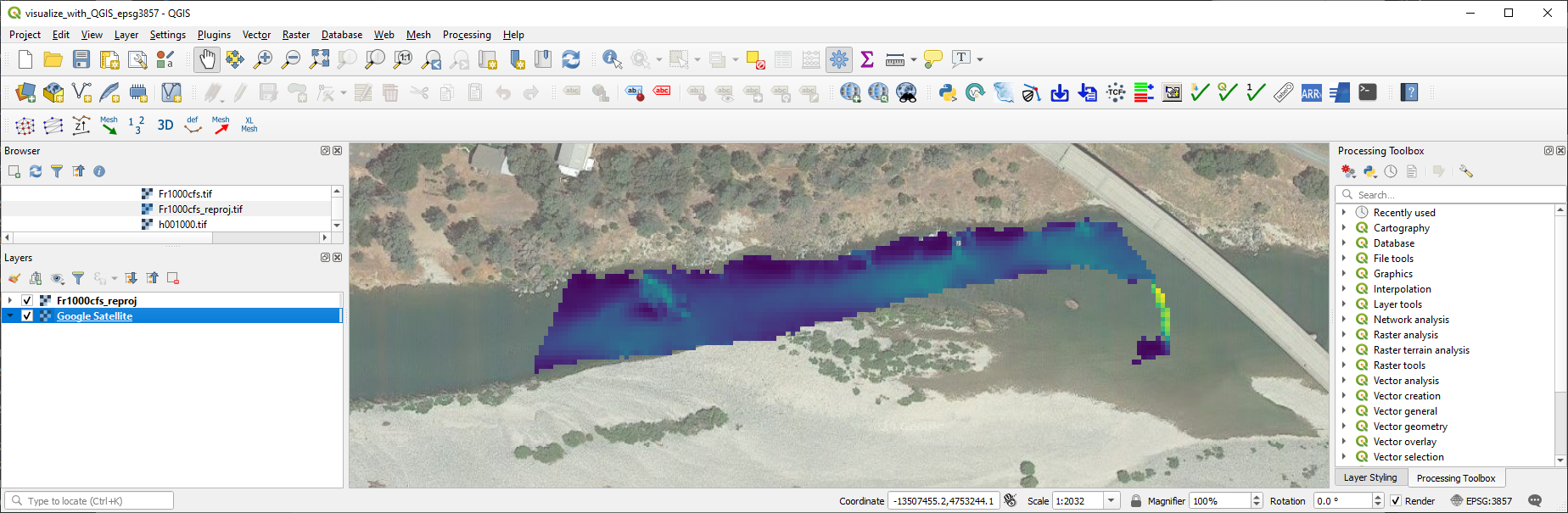
Fig. 51 The projected raster of Froude numbers.#
The reproject_raster function is also available (slightly modified) in flusstools (geotools.reproject_raster()), where saving the new reprojected raster is embedded in the function (automatically appends the syllable "_epsg[NO]" to the original file name).
Note
To display multiple rasters with different coordinate systems on the same map in QGIS, the coordinate systems must be harmonized in most cases. While QGIS will automatically propose to convert a raster with a non-project-compliant CRS to the project CRS, it also has a dedicated function for adjusting raster coordinate systems: In QGIS, click on the Raster menu > Projections > Warp (Reproject)…. Select the raster(s) to reproject (i.e., the raster(s) to harmonize with the project coordinate system). However, Warp may not perform all reprojection steps as desired and lead to wrong placements of the new raster. The Warp method is also available in Python through gdal.Warp (read the docs): kwargs={'format': 'GTiff', 'geoloc': True}gdal.Warp(TARGET_GEO_TIFF_FILE_NAME, SOURCE_GEO_TIFF_FILE_NAME, **kwargs)
Transformation errors
The coordinate transformation fails when no transformation between the indicated source and target spatial reference system can be established (i.e., gdal does not know the transformation). This problem occurs often when old, regional coordinate systems are transformed to coordinate systems for web applications (e.g., EPSG=3857). Read more in the gdal docs.
Zonal Statistics for Morphological Units#
In hydraulic and geospatial analyses, the question of statistical values of certain areas of one or more rasters often arises. For instance, we may be interested in mean values and standard deviations in specific zones of a water body. For this purpose, Zonal statistics enable the delineation of an area of a raster by using a polygon shapefile.
The River Architect dataset includes a slackwater zone and zonal statistics help to identify the mean water depth and flow velocity of slackwaters, which are a so-called morphological unit (recall the create-shapefile section).
Background
Instream morphological units aid in describing the geospatial organization of fluvial landforms, which play an important role in ecohydraulic analyses and river restoration. For instance, pool units describe deep water zones with low flow velocity, riffle units are typically characterized by shallow water depths and high velocity, and slackwater units are shallow flow zones with low flow velocity (many juvenile fish love slackwaters). Wyrick and Pasternack [WP14] introduce the delineation of morphological units and an open-access summary can be found in the Appendix Sect. 5 in Schwindt et al. [SLPR20].
To analyze a visually apparent slackwater unit, we can draw a polygon in a new shapefile that delineates morphological units. The following figures guide through the creation of a polygon shapefile and the delineation of the riffle with QGIS. Start with opening QGIS and create a new project. Import the water depth and flow velocity rasters showing the slow and shallow water zone. Then follow the workflow in the illustrations below.
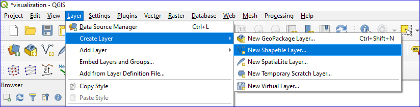
Fig. 52 QGIS: Create Layer > New Shapefile Layer…#
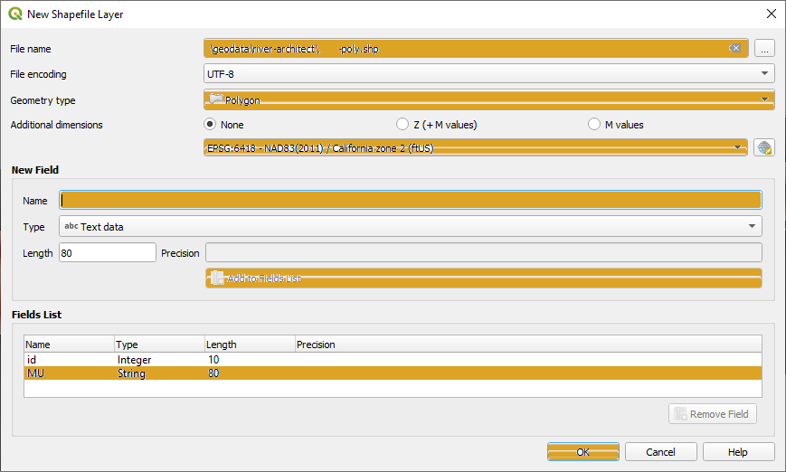
Fig. 53 Define New Shapefile Layer#
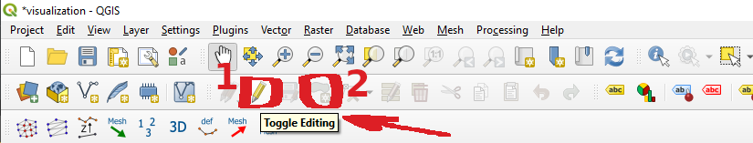
Fig. 54 Enable shapefile editing#
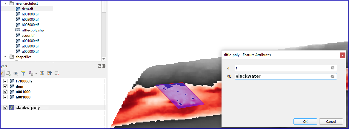
Fig. 55 Draw polygons in a shapefile in QGIS.#
Finalize the drawing by clicking on the Save Edits disk button (between Toggle Editing and Add Polygon). Just in case, the slackwater delineation polygon shapefile is also available at the jupyter-python repository of this eBook.
Recall
The new polygon is not saved as long as the edits are not saved. That means: Regularly saving edits when drawing features in QGIS.
Zonal statistics can be calculated using the gdal and ogr libraries, but this is a little cumbersome. The rasterio (conda install -c conda-forge rasterio) library provides a much more convenient method to calculate zonal statistics with its rasterstats.zonal_stats(SHP-FILE, RASTER, STATSTICS-TYPES) method. With zonal_stats, we can easily obtain statistics of the water depth and flow velocity rasters in the limits of the new slackwater polygon.
import rasterstats as rs
# make file names
h_file = r"" + os.getcwd() + "/geodata/rasters/h001000.tif"
u_file = r"" + os.getcwd() + "/geodata/rasters/u001000.tif"
zone = r"" + os.getcwd() + "/geodata/shapefiles/slackw-poly.shp"

# get water depth stats in zone
h_stats = rs.zonal_stats(zone, h_file, stats=["min", "max", "median", "majority", "sum"])
# get flow velocity stats in zone - note the different stats assignment
u_stats = rs.zonal_stats(zone, u_file, stats="min max median majority sum")

print(h_stats)
print(u_stats)
[{'min': 0.0, 'max': 5.423915386199951, 'sum': 1709.34521484375, 'median': 1.6403688192367554, 'majority': 0.0}]
[{'min': 0.0, 'max': 5.139162540435791, 'sum': 1609.26318359375, 'median': 1.879171371459961, 'majority': 0.0}]
Recall that both rasters are in the U.S. customary unit system (i.e., feet and feet per second). More statistics can be calculated with zonal_stats:
min, max, mean, count, sum, std, median, majority, minority, unique, range, nodata, percentile_<q> (where <q> can be any float number between 0 and 100).
In addition, user-defined statistics can be added, where the numpy.ma module is particularly useful with its array handling capacities, such as for transposing or specifying statistics along an axis. For instance, we can define a specific function to calculate the standard deviation as follows:
 def raster_std(raster_array):
        return np.ma.std(raster_array)
To use the raster_std function in zonal_stats, write something similar to this:
u_stats = rs.zonal_stats(
    zone, u_file,
    stats="min max",
    add_stats={"stdev": raster_std}
)
print(u_stats)
[{'min': 0.0, 'max': 5.139162540435791, 'stdev': 1.1065991101701524}]
Clip a Raster#
The above-introduced rasterstats.zonal_stats method works with “Mini-Rasters”, which represent clips of the input raster to the user-defined polygon shapefile. Moreover, a mini-raster itself can be obtained by defining the optional keyword argument raster_out=True. In the case that we want to get the original raster clipped without and statistical operation, we can use a little trick by defining an additional statistics function that returns the original array:
 def original(raster_array):
        return raster_array
With raster_out=True and the original() function, we can retrieve the clipped raster in the following array types:
mini_raster_array- a clipped and masked numpy array,mini_raster_affine- a transformation as anAffineobject (i.e., with affine 6-parameter transformation), andmini_raster_nodata-NoDatavalues.
The following code block illustrates the usage for retrieving a numpy array:
import rasterstats as rs

h_file = r"" + os.getcwd() + "/geodata/rasters/h001000.tif"
h_stats = rs.zonal_stats(zone, h_file, stats="count",
                         add_stats={"original": original},
                         raster_out=True)
print(h_stats[0].keys())
print(h_stats[0]["mini_raster_array"])
dict_keys(['count', 'original', 'mini_raster_array', 'mini_raster_affine', 'mini_raster_nodata'])
[[-- -- -- ... -- -- --]
 [-- -- -- ... -- -- --]
 [-- -- -- ... -- -- --]
 ...
 [-- -- -- ... -- -- --]
 [-- -- -- ... -- -- --]
 [-- -- -- ... -- -- --]]
Tip
Use the above-shown methods to assign a projection and save the clipped array as a GeoTIFF raster. The functions are also implemented in [flusstools] (more precisely, in [flusstools.geotools.raster_mgmt()](https://flusstools.readthedocs.io/en/latest/geotools.html#module-flusstools.geotools.raster_mgmt, which can be used as geotools.raster_mgmt()).
Slope / Aspect Maps and Built-in Command Line Scripts#
Hillslope maps are an important parameter in hydraulics, hydrology, and ecology. For instance, the slope determines the flow direction of water and it is also a criterion for delineating the habitat of many species. To calculate hill slope gradients and directions, gdal has a command-line tool called gdaldem , which requires a DEM (Digital Elevation Model) raster. The general use of gdaldem in the command line is (arguments in brackets are optional):
gdaldem slope input_dem output_slope_map [-p use percent slope (default=degrees)] [-s scale* (default=1)] [-alg ZevenbergenThorne] [-compute_edges] [-b Band (default=1)] [-of format] [-co "NAME=VALUE"]* [-q]
To call the command-line tool, we can either use a terminal/command prompt or Python’s standard library subprocess. The following code block illustrates the usage of the gdaldem command line tool through subprocess.call() to create a slope raster (in percent) from the River Architect sample data’s dem.tif. Note that subprocess.call() returns 0 if the command execution was successful and any other return value indicates an error.
import subprocess, os

cmd_create_slope = "gdaldem slope {0}/geodata/rasters/dem.tif {0}/geodata/rasters/slope-percent.tif -p".format(os.path.abspath(""))
subprocess.call(cmd_create_slope, shell=True)
0
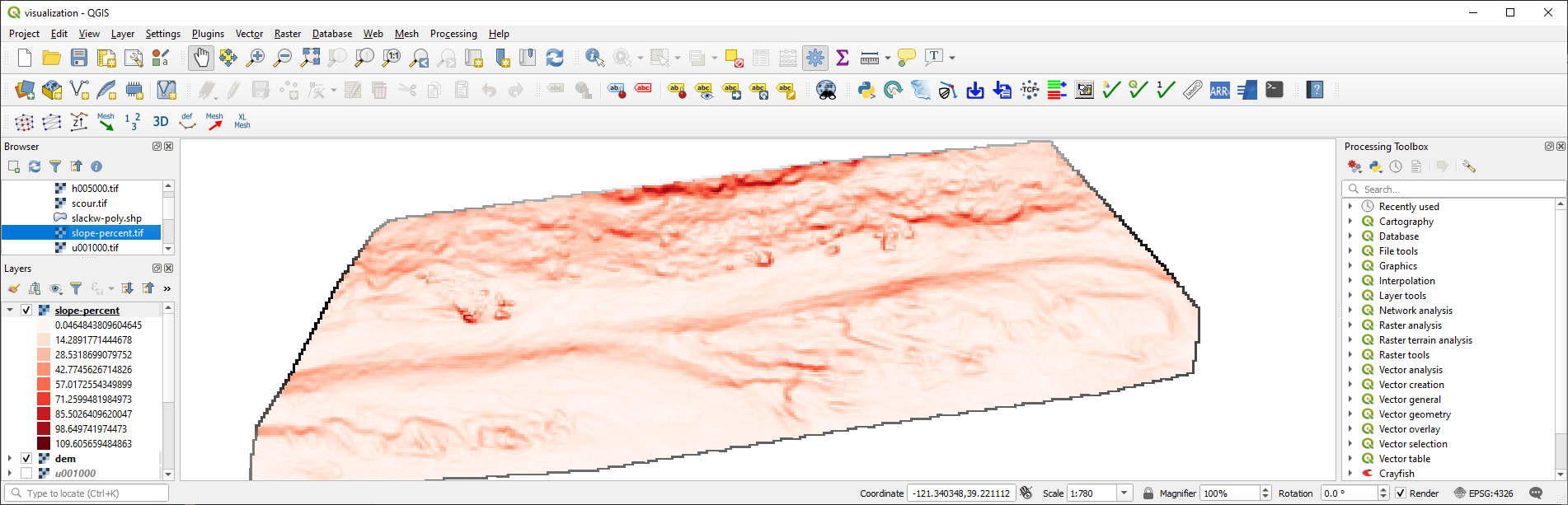
Fig. 56 The new slope raster.#
In addition to the absolute slope (i.e., inclination in degrees), or instead of the slope, it can be important to know the slope direction (e.g., inclination toward south, west, east, or north). A raster indicating the slope direction is called aspect raster, where south corresponds to 0° (and 360°), west to 90°, north to 180°, and east to 270°. An aspect raster can also be created with gdaldem:
gdaldem aspect input_dem output_aspect_map [-trigonometric] [-zero_for_flat] [-alg ZevenbergenThorne] [-compute_edges] [-b Band (default=1)] [-of format] [-co "NAME=VALUE"]* [-q]
To create an aspect raster of the River Architect sample data DEM run:
cmd_create_aspect = "gdaldem aspect {0}/geodata/rasters/dem.tif {0}/geodata/rasters/slope-aspect.tif".format(os.path.abspath(""))
subprocess.call(cmd_create_aspect, shell=True)
0
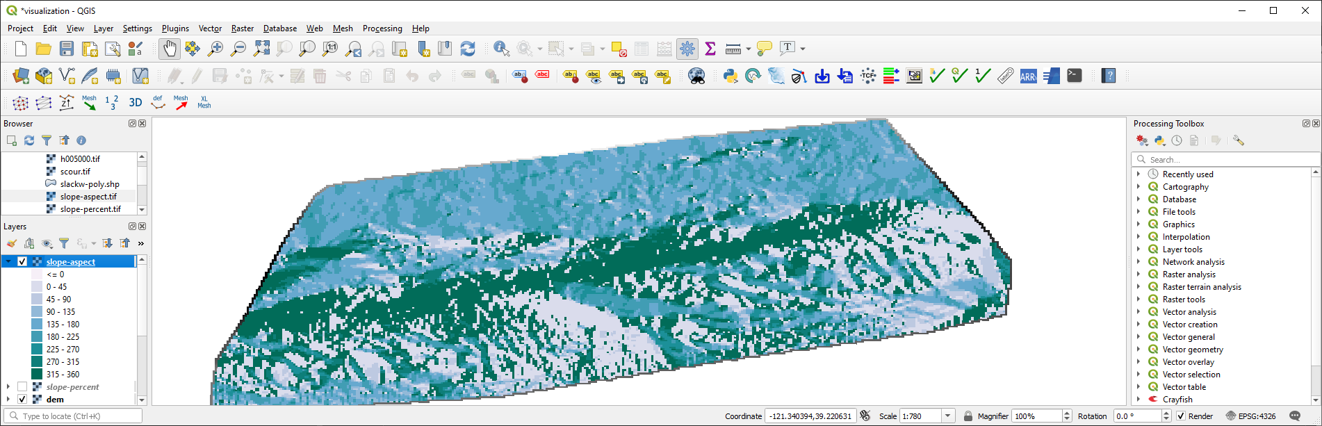
Fig. 57 The new aspect raster.#
Least Cost Path between Pixels (and another Way of Reprojection)#
Ecohydraulic Background#
Least cost paths are important to plan efficient routes for navigation (e.g., in a car) and they can also be helpful in ecohydraulics. Let’s take for a moment the position of a fish that, after a flood with decreasing discharge, wants to swim as fast as possible from the floodplain back into the main channel where there is enough water. In the figure below, point 1 shows the starting point on the floodplain and point 2 the destination in the main channel. The reddish background represents the above-produced slope raster (slope-percent.tif) and the water depth at average annual discharge is colored in blue.
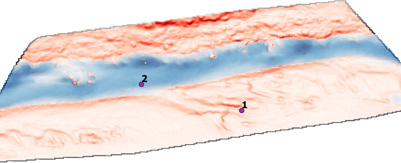
Fig. 58 The slope raster with points 1 and 2 highlighted.#
Naturally, the path of least costs corresponds to the path of the steepest, monotonously downward-facing slope and we will assume that a fish is able to find it.
Note
In many rivers, fish face the daily challenge of escaping from the deadly trap of lateral depressions. The reason for this is that many hydroelectric power plants cause abrupt fluctuations in discharge due to fluctuations in energy demand and production (so-called hydro-peaking). As a result, there is a high stranding risk for fish in many regulated rivers that are subjected to hydro-peaking. The following figure illustrates stranding risk zones as a function of discharge (in cubic feet per second) at the lower Yuba River (California, USA).
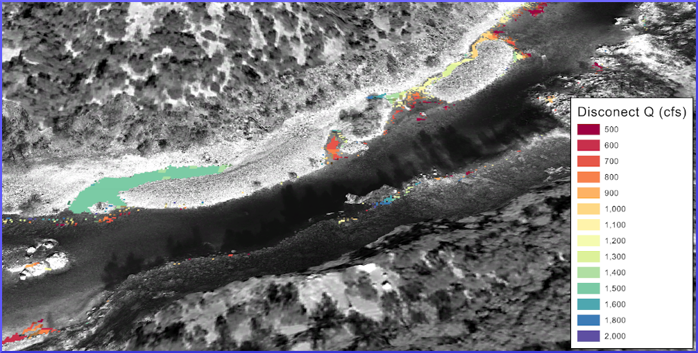
Fig. 59 Fish stranding map created with River Architect (source: the River Architect Wiki / Kenneth Larrieu](https://riverarchitect.github.io/RA_wiki/StrandingRisk)).#
Functions and Libraries Involved#
The skimage (scikit-image) library (cf. Other packages in the Open source libraries section) provides with skimage.graph.route_through_array a smart method to calculate the least cost path by summing up pixel-wise connections from point 1 to point 2.
Here is how it works: Assume a numpy array (e.g., with random slope values) that looks like this:
slope_image = np.random.randint(100, size=(3, 5))
slope_image
array([[58,  0, 85, 47, 46],
       [91, 64, 79, 25, 46],
       [88, 24,  3, 96, 31]])
To find the fastest way from array index [0][0] (top left point_1 = (0, 0)) to array index [2][4] (bottom right point point_2 = (2, 4)), we can use route_through_array() to get a list (least_cost_path_indices) with the array coordinates of the path to go, and the costs (weight) involved (sum of all pixels of the least cost path):
from skimage.graph import route_through_array

point_1 = (0, 0)
point_2 = (2, 4)
least_cost_path_indices, weight = route_through_array(slope_image, point_1, point_2)
least_cost_path_indices, weight
([(0, 0), (0, 1), (1, 1), (2, 2), (1, 3), (2, 4)], 167.7731239591687)
To integrate the least cost path list into an array that we can rasterize (geotools.create_raster()), we can paste least_cost_path_indices into a numpy-zeros array of the original slope raster (image) as a transposed list.
least_cost_path_indices = np.array(least_cost_path_indices).T
least_cost_path_array = np.zeros_like(slope_image)
least_cost_path_array[least_cost_path_indices[0], least_cost_path_indices[1]] = 1
least_cost_path_array
array([[1, 1, 0, 0, 0],
       [0, 1, 0, 1, 0],
       [0, 0, 1, 0, 1]])
In practice, the slope raster is georeferenced, and therefore, we have to use pixel coordinates relative to the coordinate system origin. For this purpose, we need two more functions:
One function to calculate the pixel-index related offset that we will name
coords2offset: Thecoords2offset()function will return the x-y shift in the form of “number of pixels” (two integers, one for x and one for y shift).The above-defined get_srs() function (i.e.,
geotools.get_srs()).
The coords2offset() function looks like this:
def coords2offset(geo_transform, x_coord, y_coord):
    """
    Returns x-y pixel offset
    :param geo_transform: osgeo.gdal.Dataset.GetGeoTransform() object
    :param x_coord: FLOAT of x-coordinate
    :param y_coord: FLOAT of y-coordinate
    :return: offset_x, offset_y (both integer of pixel numbers)
    """
    origin_x = geo_transform[0]
    origin_y = geo_transform[3]
    pixel_width = geo_transform[1]
    pixel_height = geo_transform[5]
    offset_x = int((x_coord - origin_x) / pixel_width)
    offset_y = int((y_coord - origin_y) / pixel_height)
    return offset_x, offset_y
Tip
The coords2offset() function is also available in flusstools with more robust raise-exception notation: use with geotools.coords2offset() and have a look into the script located in flusstools.geotools.dataset_mgmt.
The coords2offset() function converts a raster array (e.g., produced with the above-defined geotools.raster2array() function) into an array that can be used with route_through_array() with the following workflow:
Use the raster’s
geo_transform(gdal.Dataset.GetGeoTransform = (origin_x, pixel_width, 0, origin_y, 0, pixel_height)) and the start and end point coordinates (i.e,start_coordof point 1 andstop_coordof point 2) incoords2offset()to get their pixel indices (start_index_x,start_index_y,stop_index_x, andstop_index_y) in the raster array.Replace
np.nanvalues in the raster array with values that are higher than the maximum value of the array. Do not use zeros, because we want to exclude thenp.nanpixels from the least cost path later by overwritingnp.nanwith very high pixel costs.Use
route_through_array()as above explained with the optional argumentsgeometric=True(use the MCP_Geometric class rather than MCP_base to calculate costs) andfully_connected=True(enables using diagonal pixels as direct neighbors).Integrate the least cost path list (
index_path) into a numpy-zeros array (child ofraster_array, as explained above) and return thepath_array.
def create_path_array(raster_array, geo_transform, start_coord, stop_coord):
    # transform coordinates to array index
    start_index_x, start_index_y = coords2offset(geo_transform, start_coord[0], start_coord[1])
    stop_index_x, stop_index_y = coords2offset(geo_transform, stop_coord[0], stop_coord[1])

    # replace np.nan with max raised by an order of magnitude to exclude pixels from least cost
    raster_array[np.isnan(raster_array)] = np.nanmax(raster_array) * 10

    # create path and costs
    index_path, cost = route_through_array(raster_array, (start_index_y, start_index_x),
                                               (stop_index_y, stop_index_x),
                                               geometric=True, fully_connected=True)


    index_path = np.array(index_path).T
    path_array = np.zeros_like(raster_array)
    path_array[index_path[0], index_path[1]] = 1
    return path_array
Application#
Recall, we defined the following functions (all are available in flusstools through from flusstools import geotools) that we can use for the calculation of the least cost path to get from point 1 to point 2 in the slope-percent.tif raster:
geotools.raster2array()geotools.create_path_array()geotools.get_srs()geotools.create_raster()
The below code block uses these functions as follows:
Define input (slope-percent.tif) and output (least_cost.tif) raster names (with directories).
Define the coordinates of points 1 and 2 as tuples (x, y) in the EPSG:6418 projection.
Load the input raster(
src_raster), its band as array (raster_array), and geotransformation (geo_transform) with theraster2array()function.Get the least cost path indicated with ones in an array of zeros ( i.e., an on-off
path_array) with thecreate_path_array()function.Get the
osgeo.osr.SpatialReferenceof the input raster (src_raster = osgeo.gdal.Dataset("slope-percent.tif")).Create the least cost path GeoTIFF raster with the
create_raster()function as agdal.GDT_Byteband.
from skimage.graph import route_through_array

# define raster input and out names
in_raster_name = r"" + os.path.abspath("") + "/geodata/rasters/slope-percent.tif"
out_raster_name = r"" + os.path.abspath("") + "/geodata/rasters/least_cost.tif"
# define coordinates of points 1 and 2 (in EPSG:6418)
point_1_coord = (6749261.94092826917767525, 2206970.35179582564160228)
point_2_coord = (6749016.82820663042366505, 2207050.61491037486121058)

# get source raster (osgeo.gdal.Dataset), the raster as nd.array, and the geotransformation tuple
src_raster, raster_array, geo_transform = raster2array(in_raster_name)
# get the zeros-like array with least cost pixels = 1
path_array = create_path_array(raster_array, geo_transform, point_1_coord, point_2_coord)
# get the spatial reference system of the input raster (slope-percent.tif)
src_srs = get_srs(src_raster)
# project the least cost path_array into a Byte (only zeros and ones) raster
create_raster(out_raster_name, path_array, epsg=int(src_srs.GetAuthorityCode(None)),
              rdtype=gdal.GDT_Byte, geo_info=geo_transform)
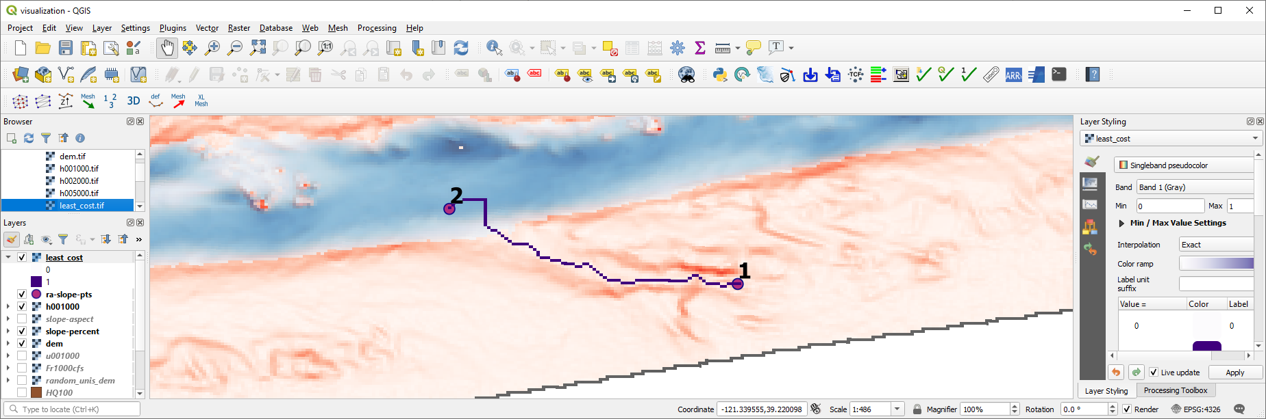
Fig. 60 The least cost path illsutrated in QGIS.#
Legitimately, you may wonder whether it was better to represent the least cost path as a line. Of course, that is correct. However, this operation is a conversion of a raster into a line shapefile, which is explained in the next section on geodata conversion. Curious readers can also directly use the raster2line() function of flusstools (or have a look at it in the flusstools.geotools/dataset_mgmt.py script).
Exercise
Familiarize with raster handling in the geospatial ecohydraulics exercise.