Bedload

Bedload#

Bedload basics

Bedload traveling in a lab flume by jumping, rolling, and sliding (under water footage). Source: Sebastian Schwindt@ Hydro-Morphodynamics channel on YouTube.

For a better learning experience, the Glossary helps with explanations of the terms Sediment transport, (dimensionless) bedload transport $Φ_{b}$ , dimensionless bed shear stress $τ_{x}$ , and the Shields parameter $τ_{x, c r}$ (in this order).

Sediment replenishment, gravel augmentation, bedload addition (etc.)

The placement of coarser sediment for the restoration of bedload transport can take many different forms and it is described by a broad range of terms. In TELEMAC, the best option for simulating such bedload restoration efforts is the Nestor module that requires Gaia (or SISYPHE). Read more in the most recent Nestor manual.

Principles#

The calculation of bedload transport requires expert knowledge about the modeled ecosystem for judging whether the system is sediment supply-limited or transport capacity-limited [CF15].

Sediment supply-limited rivers: A sediment supply-limited river is characterized by clearly visible incision trends indicating that the river’s runoff could potentially transport more sediment than is available in the river. Sediment-supply limited river sections typically occur downstream of dams, which represent an insurmountable barrier for sediment. Thus, in a supply-limited river, the flow competence (hydrodynamic force or transport capacity) is insufficient to mobilize a typically coarse riverbed, but it is sufficient for transporting external sediment supply.
Transport capacity-limited (alluvial) rivers: A transport capacity-limited river is characterized by sediment abundance where the river’s runoff is too small to transport all available sediment during a flood. Sediment accumulations (i.e., the alluvium) are present and the channel tends to braid into anabranches. Thus, the flow competence (or transport capacity) is insufficient to transport the entire amount of available sediment (external supply and riverbed).

Limitation types vary in space and in time

The channel types may strongly vary in space between river sections or segments and in time. For instance, the same river section that appears to be supply-limited because of insufficient flow competence may turn into a transport capacity-limited section during a flood when high discharges exert high shear stresses on the riverbed. The spatio-temporal variation of transport limitation types is particularly pronounced in near-census, healthy river ecosystems that are perpetually adjusting to a morphodynamic equilibrium.

The following figures feature sediment supply-limited river sections and a transport capacity-limited river section.

Artificially sediment supply-limited

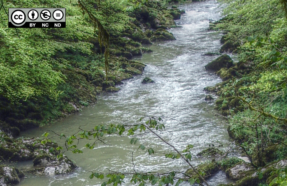
channel doubs france sediment supply transport limited — Fig. 193 The Doubs in the Franche-Comté (France) during a small flood. The sediment supply is interrupted by a cascade of dams upstream with the consequence of a straight monotonous channel with significant plant growth along the banks. The riverbed primarily consists of boulders that are immobile most of the time. Thus, the river section can be characterized as artificially sediment supply-limited (picture: Sebastian Schwindt 2015).#

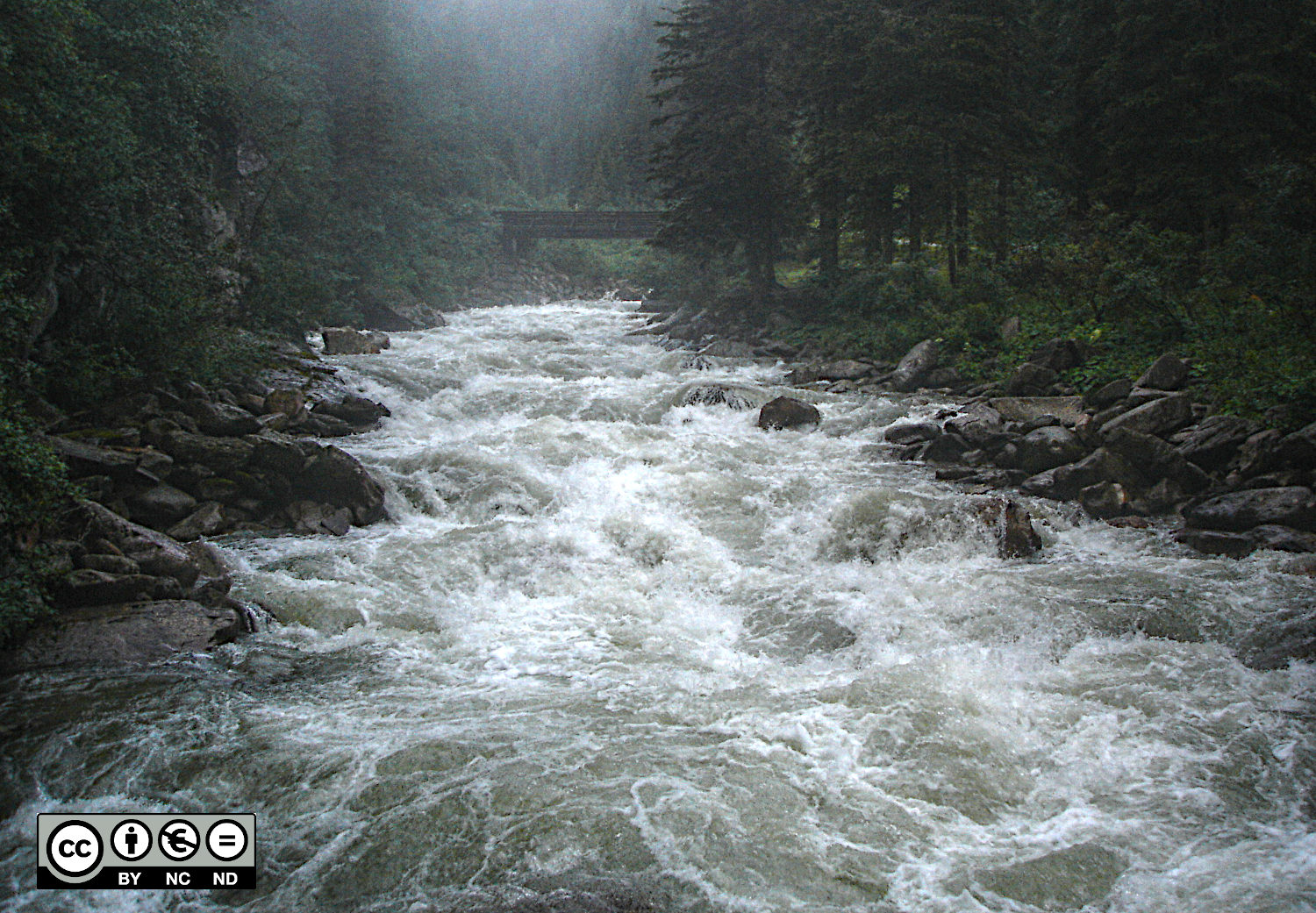
Naturally sediment supply-limited

naturally channel krimmler ache austria sediment supply transport limited — Fig. 194 The Krimmler Ache in Austria during a small flood event. Even though the watershed has a high Sediment yield, the transport capacity of the water in this river section is so high that the riverbed predominantly consists of large boulders. Thus, the river section can be characterized as naturally sediment supply-limited (picture: Sebastian Schwindt 2010).#

Capacity-limited

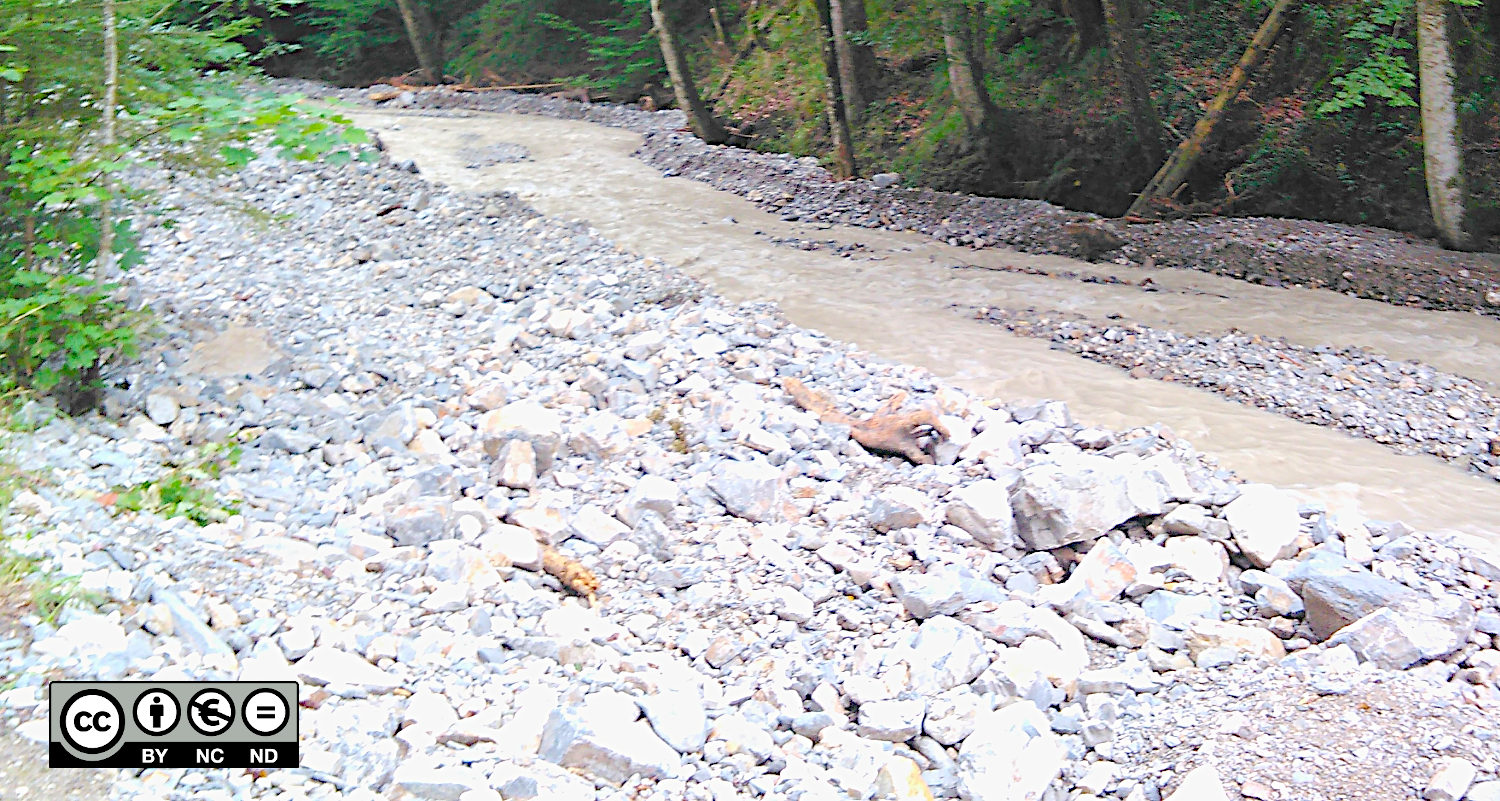
alluvial channel jenbach sediment supply transport limited — Fig. 195 The Jenbach in the Bavarian Alps (Germany) after an intense natural sediment supply in an upstream reach in the form of a landslide. The river section can be characterized as transport capacity-limited (picture: Sebastian Schwindt 2020).#

Why is the differentiation between sediment supply and transport capacity-limited rivers important for numerical modeling?

Gaia provides different formulae for calculating bedload transport, which are partially either derived from lab experiments with infinite sediment supply (e.g., the Meyer-Peter and Müller [MPM48] formula and its derivates, see below) or from field measurements in partially transport capacity-limited rivers (e.g., Wilcock [Wil93]). Formulae that account for limited sediment supply often involve a correction factor for the Shields parameter.

Formulae and Parameters#

Bedload is typically designated with $q_{b}$ (in kg $\cdot$ s $^{- 1} \cdot$ m $^{- 1}$ i.e. weight per unit time and width) and accounts for particulate transport in the form of the displacement of rolling, sliding, and/or jumping coarse particles. In river hydraulics, the so-called Dimensionless bed shear stress, also referred to as Shields parameter [Shi36], is often used as a threshold value for the mobilization of sediment from the riverbed. TELEMAC and Gaia build on a dimensionless expression of bedload transport intensity according to Einstein [Ein50]:

(2)#

Φ_{b} = \frac{q_{b}}{ρ_{s} \sqrt{(s - 1) g D_{p q}^{3}}}

where $ρ_{s}$ is the density of sediment grains; $s$ is the ratio of sediment grain and water density (typically 2.68) [Sch17]; $g$ is gravitational acceleration; and $D_{p q}$ is the characteristic grain diameter of the sediment class (cf. Sediment Classes). Note that the dimensionless expression $Φ$ and the dimensional expression $q_{b}$ represent unit bedload (i.e., bedload normalized by a unit of width). Gaia outputs are dimensional and correspond to $q_{b}$ (recall the VARIABLES FOR GRAPHIC PRINTOUTS definitions in the General Parameters section) where the unit of width corresponds to the edge length of a numerical mesh cell over which the mass fluxes are calculated.

Comment on the Original Einstein (1950) Expression

The original equation for $Φ_{b}$ can be found on page 34 (Equation 42) in Einstein [Ein50]. This formula involves an additional division by the gravitational acceleration $g$ , which does not appear in later references to the Einstein expression of $Φ_{b}$ and would also not result in a dimensionless term. For this reason, Equation (2) is adapted here.

Equation (2) expresses only the dimensional conversion for bedload transport (i.e., the way how dimensions are removed or added to sediment transport). In fact, this is only the first step to solve the other side of a bedload equation using a (semi-) empirical formula. To calculate $Φ_{b}$ , Gaia provides a set of (semi-) empirical formulae, which can be modified with user Fortran files and defined in the Gaia steering file with the BED-LOAD TRANSPORT FORMULA FOR ALL SANDS integer keyword. Table 10 lists possible integers for the keyword to define a bedload transport formulae, including references to original publications, formula application ranges, and the names of the Fortran source files for modifications.

Table 10 Bedload transport formulae implemented in Gaia with application limits regarding the grain diameter $D$ , **cross section-averaged** Froude number $F r$ , slope $S$ , water depth $h$ , and flow velocity $u$ . The Fortran files live in the TELEMAC source/gaia directory.#
Gaia	Author(s)	$D$	Fr; $S$ ; $h$ ; and $u$	User Fortran
(no.)	(ref.)	(10 $^{- 3}$ m)	(-); (-); (m); (m/s)	(file name)
`1`	Meyer-Peter and Müller [MPM48]	0.4 $< D_{50} <$ 28.6	10 $^{- 4} < F r <$ 639 0.0004 $< S <$ 0.02 0.01 $< h <$ 1.2 0.2 $< u$	bedload_meyer_gaia.f
`2`	Einstein [Ein50]-Brown [Bro49]	0.25 $< D_{35} <$ 32		bedload_einst.f
`3`	Engelund and Hansen [EH67]	0.15 $< D_{50} <$ 5.0	0.1 $< F r <$ 10	bedload_engel_gaia.f
`30`	Chollet and Cunge [CC79], Engelund and Hansen [EH67]	0.15 $< D_{50} <$ 5.0	0.1 $< F r <$ 10	bedload_engel_cc_gaia.f
`7`	Van Rijn [VR84b]	0.6 $< D_{50} <$ 2.0	0.5 $< h$ 0.2 $< u$	bedload_vanrijn_gaia.f
`10`	Wilcock and Crowe [WC03]	0.063 $≲ D_{p q}$		bedload_wilcock_crowe_gaia.f

To use the Meyer-Peter and Müller [MPM48] formula (1 according to Tab. 10) in this tutorial, add the following line to the gaia-morphdynamics.cas steering file:

/ continued: gaia-morphodynamics.cas
/
/ BEDLOAD
/
BED LOAD FOR ALL SANDS : YES / deactivate with NO
BED-LOAD TRANSPORT FORMULA FOR ALL SANDS : 1

The following sections provide more details on how $Φ_{b}$ is calculated with the pre-defined formulae listed in Tab. 10.

User-defined Bedload transport formulae in a specific Fortran file

Users can add more bedload transport formulae by adding a modified copy of a FORTRAN file template. The Gaia manual explains the procedure for adding a new user-defined bedload formula in detail in section 6.3.

User Fortran Files

To implement a user Fortran file, copy the original TELEMAC Fortran file from the /telemac/v9.0.0/sources/ directory (e.g., /telemac/v9.0.0/sources/gaia/bedload_einst_gaia.f) to the project directory (e.g., /telemac/v9.0.0/simulations/gaia-tutorial/user_fortran/bedload_einst_gaia.f). Finally, tell TELEMAC where to look for user fortran files by defining the following keyword in a steering file (e.g., in gaia-morphodynamics.cas):

FORTRAN FILE : 'user_fortran'

Meyer-Peter and Müller (1948)#

Recall the validity range for the MPM formula (1)

Revise Tab. 10 to ensure that the application is in the applicable range of parameters corresponding to the conditions under which the formula has been developed.

The Meyer-Peter and Müller [MPM48] formula was published in 1948 by Swiss researchers Eugen Meyer-Peter, professor at ETH Zurich and founder of the school’s hydraulics laboratory (Zurich’s famous VAW), and Robert Müller. Their empirical formula is the result of more than a decade of collaboration and the elaboration began one year after the VAW was founded in 1931 when Robert Müller was appointed assistant to Eugen Meyer-Peter. The two scientists also worked with Henry Favre and Hans-Albert Einstein who came up with another approach for calculating bedload. An early version of the Meyer-Peter and Müller [MPM48] formula was published in 1934 and it is the basis for many other formulas that refer to a critical Dimensionless bed shear stress (i.e., Shields parameter). It is important to remember that the formula is based on data from lab flume experiments with high sediment supply. This is why bedload transport calculated with the Meyer-Peter and Müller [MPM48] formula corresponds to the hydraulic transport capacity of an alluvial channel. Thus, the Meyer-Peter and Müller [MPM48] formula tends to overestimate bedload transport and it is inherently designed for estimating bedload based on simplified 1d cross section-averaged hydraulics (see also the Python sediment transport exercise). Good results can be expected when flood flows are simulated in an alluvial river section.

Ultimately, the left side of Equation (2) ( $Φ_{b}$ ) can be calculated with the Meyer-Peter and Müller [MPM48] formula as follows:

(3)#

\begin{array}{r} Φ_{b} = {\begin{cases} 0 & if τ_{x, c r} > τ_{x} \\ f_{m p m} \cdot (τ_{x} - τ_{x, c r})^{3 / 2} & if τ_{x, c r} \leq τ_{x} \end{cases} \end{array}

where $f_{m p m}$ is the MPM coefficient (default is 8), $τ_{x, c r}$ denotes the Shields parameter ( $\approx$ 0.047 and up to 0.07 in mountain rivers), and $τ_{x}$ is the Dimensionless bed shear stress. When using the Meyer-Peter and Müller [MPM48] formula with Gaia, consistency with original publications is ensured by defining $τ_{x, c r}$ and $f_{m p m}$ in the steering file:

/ continued: gaia-morphodynamics.cas
/
/ BEDLOAD
BED-LOAD TRANSPORT FORMULA FOR ALL SANDS : 1 / see above
CLASSES SHIELDS PARAMETERS : 0.047;0.047;0.047
MPM COEFFICIENT : 8

Wong-Parker correction of the MPM formula

The Wong-Parker [WP06] correction for the Meyer-Peter and Müller [MPM48] formula refers to a statistical re-analysis of the original experimental datasets and applies to Plane bed river sections. To this end, the Wong-Parker correction yields lower bedload transport values and it excludes the form drag correction of the original formula with the following expression: $Φ_{b} \approx 3.97 \cdot (τ_{x} - 0.0495)^{3 / 2}$ . Thus, to implement the Wong-Parker correction in Gaia use:

CLASSES SHIELDS PARAMETERS : 0.0495;0.0495;0.0495
MPM COEFFICIENT : 3.97

To directly continue with the tutorial using the Meyer-Peter and Müller [MPM48] formula, jump to the correction factors section.

Einstein-Brown (1942/49)#

Recall the validity range for the Einstein-Brown formula (2)

Revise Tab. 10 to ensure that the application is in the applicable range of parameters corresponding to the conditions under which the formula has been developed.

Hans Albert Einstein, son of the famous Albert Einstein, was a pioneer of probability-based analyses of sediment transport. In particular, he hypothesized that the beginning and the end of sediment motion can be expressed in terms of probabilities. Furthermore, Einstein assumed that sediment motion is a series of step-wise displacements followed by rest periods and that the average distance of a particle displacement is approximately a hundred times the particle (grain) diameter. Moreover, to account for observations he made in lab flume experiments, Einstein introduced hiding and lifting correction coefficients [Ein42].

The Einstein formula differs from any Meyer-Peter and Müller [MPM48]-based formula in that it does not imply a threshold for incipient motion of sediment. However, despite or because Einstein’s sediment transport theory is more complex than many other bedload transport formulae, it did not become very popular in engineering applications. Today, Gaia enables the user-friendly application of Einstein’s formula, which was similarly presented by Brown [Bro49] at an engineering hydraulic conference in 1949. According to Einstein [Ein42]-Brown [Bro49], the left side of Equation (2) ( $Φ_{b}$ ) is calculated as follows:

(4)#

\begin{array}{r} Φ_{b} = {\begin{cases} 0 & if τ_{x} < 0.0025 \\ F_{e b} \cdot 2.15 \cdot \exp (- 0.391 / τ_{x}) & if 0.0025 \leq τ_{x} \leq 0.2 \\ F_{e b} \cdot 40 \cdot τ_{x}^{3} & if τ_{x} > 0.2 τ_{x} \end{cases} \end{array}

where

(5)#

F_{e b} = {(\frac{2}{3} + \frac{36}{D_{x}})}^{0.5} - {(\frac{36}{D_{x}})}^{0.5}

$D_{x}$ is the dimensionless particle diameter calculated as:

(6)#

D_{x} = {[\frac{(s - 1) \cdot g}{ν^{2}}]}^{1 / 3} \cdot D_{p q}

where $s$ is the ratio of sediment grain and water density (typically 2.68); $g$ is gravitational acceleration; and $ν$ is the kinematic viscosity of water ( $\approx$ 10 $^{- 6}$ m $^{2}$ s $^{- 1}$ ) [Sch17].

To use the Einstein [Ein42]-Brown [Bro49] formulae in Gaia use:

BED-LOAD TRANSPORT FORMULA FOR ALL SANDS : 2

Consider adapting bedload_einst.f

The application thresholds as a function of $τ_{x}$ stem from the Gaia Fortran file bedload_einst.f. However, the original Einstein [Ein42]-Brown [Bro49] publications suggest a threshold of $τ_{x}$ =0.182 (rather than 0.2) for switching the formula cases.

Engelund-Hansen (1967) / Chollet-Cunge#

Recall the validity range for the Engelund-Hansen formulae (3 and 30)

Revise Tab. 10 to ensure that the application is in the applicable range of parameters corresponding to the conditions under which the formula has been developed.

The Engelund and Hansen [EH67] formula accounts for total sediment transport including Bedload and Suspended load. Starting from the Bagnold power-approach [Bag66, Bag80], the Engelund and Hansen [EH67] formula was developed for sediment transport calculations over dune channel beds. The approach accounts for energy losses required to drive particles uphill on dunes of the riverbed. The Bagnold [Bag66] theory considers the total shear as the sum of the shear transmitted between grains and the fluid, and the shear transmitted by momentum changes caused by intergranular collisions. Thus, erosion takes place as long as the Dimensionless bed shear stress is greater or equal to its critical value (i.e., the Shields parameter). Gaia implements the Engelund and Hansen [EH67] by calculating the left side of Equation (2) ( $Φ_{b}$ ) as follows:

(7)#

Φ_{b} = 0.05 \cdot \frac{f_{e h}^{2.5}}{c_{f}}

where $c_{f}$ is a friction coefficient that accounts for form drag and skin friction (calculated with the hydrodynamics in Telemac2d/3d). Read more about skin friction in the correction factors section. The $f_{e h}$ factor is a function of the Dimensionless bed shear stress $τ_{x}$ . To use the Engelund and Hansen [EH67] formula in Gaia use:

BED-LOAD TRANSPORT FORMULA FOR ALL SANDS : 30

In addition, Chollet and Cunge [CC79] introduced a step-wise function for the calculation of $f_{e h}$ :

(8)#

\begin{array}{r} f_{e h} = {\begin{cases} 0 & if τ_{x} \leq 0.06 & (no transport) \\ [2.5 (τ_{x} - 0.06)]^{0.5} & if 0.06 < τ_{x} < 0.384 & (dunes) \\ 1.066 \cdot τ_{x}^{0.176} & if 0.384 < τ_{x} < 1.08 & (transitional) \\ τ_{x} & if 1.08 \leq τ_{x} & (sheet flow) \end{cases} \end{array}

To apply the correction Chollet and Cunge [CC79] adaption of the Engelund and Hansen [EH67] formula use:

BED-LOAD TRANSPORT FORMULA FOR ALL SANDS : 3

van Rijn (1984)#

Recall the validity range for the van-Rijn formula (7)

Revise Tab. 10 to ensure that the application is in the applicable range of parameters corresponding to the conditions under which the formula has been developed.

The sediment transport formula from Leo van Rijn [VR84b] is inspired by the theories from Bagnold [Bag80], Einstein [Ein42], and Ackers and White [AW73]. The Van Rijn [VR84b] formulae assume that bedload is dominated by gravity while suspended load transport is controlled by turbulence according to Bagnold [Bag80]. To this end, the Van Rijn [VR84b] formulae calculate bedload transport similar to Ackers and White [AW73] where transport rates depend on friction velocities. To calibrate his near-bed (bedload) solid transport model, Van Rijn [VR84b] used data from experiments on flat-bed (zero-slope) channels with an average sediment grain diameter of 1.8 mm. Van Rijn [VR84b] conducted additional experiments to vet the results of his model against varying grain diameters between 0.2 and 2 mm. In addition, Van Rijn [VR84b] established criteria for sediment suspension based on laboratory experiments with grain diameters of less than 0.5 mm and by simplifying calibration parameters empirically. While the original Van Rijn [VR84b] formula accounts for total sediment transport (i.e., Bedload and Suspended load), the following explanations for the implementation in Gaia are limited to Bedload only.

According to Van Rijn [VR84b], the left side of Equation (2) ( $Φ_{b}$ ) is calculated as follows:

(9)#

Φ_{b} = \frac{0.053}{D_{x}^{0.3}} \cdot {(\frac{τ_{x} - τ_{x, c r}}{τ_{x, c r}})}^{2.1}

Explanations of the Dimensionless bed shear stress $τ_{x}$ , its critical value $τ_{x, c r}$ (i.e., the Shields parameter), and the dimensionless grain diameter $D_{x}$ are provided in the above sections on the Meyer-Peter and Müller and the Einstein-Brown formulae.

To use the Van Rijn [VR84b] formula in Gaia use:

BED-LOAD TRANSPORT FORMULA FOR ALL SANDS : 7

Wilcock-Crowe (2003)#

Applicability of the Wilcock-Crow formula (10)

The multi-fraction bedload transport formula from Wilcock and Crowe [WC03] does not state particular validity ranges, but the authors restrict their approach to sand-gravel-cobble sediments with a minimum grain diameter of 0.063 mm. The explanations in this section limit to the application background of the Wilcock and Crowe [WC03] approach. The complex set of equations is explained in detail in the Gaia manual (section 3.1.2) and by Cordier et al. [CTC+19], Cordier et al. [CTC+20].

The Wilcock and Crowe [WC03] approach is a multi-fraction sediment transport model that is primarily applicable in armored river sections for modeling bed aggradation or degradation. The approach takes up the idea of Parker [Par90] on applying a reference shear stress at which little but constant solid transport rate can be observed. The reference shear stress is close to, but a little bit larger than the Shields parameter $τ_{x, c r}$ . To this end, Wilcock and Crowe [WC03] implement a reference transport rate of 0.002 as proposed by Parker [Par90].

Moreover, the multi-fraction Wilcock and Crowe [WC03] model uses the complete sediment grain size distribution of the riverbed surface and calculates bedload transport for each of the specified grain size classes (starting with the smallest grain size). The sediment transport model builds on flume experiments from Proffitt and Sutherland [PS83] and Parker [Par90], and it accounts for hiding/exposure effects on gravel transport as a function of the sand fraction in the riverbed.

In a nutshell, the Wilcock and Crowe [WC03] model represents a further development of the Meyer-Peter and Müller [MPM48] formula, takes up the implementation of a reference transport rate [Par90], and it is calibrated to hiding/exposure effects as a function of the sand fraction.

The calculation of Bedload transport according to Wilcock and Crowe [WC03] starts with a definition of a dimensionless transport capacity $Φ_{i}$ per sediment fraction that removes dimensions from the bedload transport rate computed with a third-party formula for that fraction only (e.g., the Meyer-Peter and Müller [MPM48] formula).

To use the Wilcock and Crowe [WC03] formula in Gaia, define multiple sediment classes and use:

BED-LOAD TRANSPORT FORMULA FOR ALL SANDS : 10

Correction Factors#

Correction factors for sediment transport may be needed to account for transversal channel slope, secondary currents, or skin friction correction.

Friction Correctors#

Friction is often considered with simplified approaches lumping together skin friction and form drag, but in a two-dimensional model, only skin friction affects bedload. Einstein [Ein50] accounts for skin friction with a correction factor $f_{f r}$ for (dimensional) bed shear stress $τ$ :

(10)#

τ^{'} = f_{f r} \cdot τ

How Telemac2d calculates $τ$

Telemac2d uses the length of the $x$ - $y$ velocity vectors to calculate $τ$ with the user-defined FRICTION COEFFICIENT $c_{f}$ : $τ = 0.5 \cdot ρ_{w} \cdot c_{f} \cdot (U^{2} + V^{2})$ .

The correction factor $f_{f r}$ is defined as the ratio of the global friction coefficient $c_{f}$ (i.e., lumped skin friction and form drag) and the skin friction-only coefficient $c_{f}^{'}$ :

(11)#

f_{f r} = \frac{c_{f}^{'}}{c_{f}}

The skin friction-only coefficient is calculated as:

(12)#

c_{f}^{'} = 2 \cdot {(\frac{κ}{l o g (12 h / k_{s}^{'})})}^{2}

where $κ$ is the Von Karmàn [VK30] constant (0.4), $h$ is water depth, and $k_{s}^{'}$ is the representative roughness length, which is often assumed as a multiple of the characteristic grain size (read more in the section on bedload calibration).

Skin Friction

Gaia uses by default the skin friction correction coefficient that it derives from the hydrodynamic solver (i.e., Telemac2d/3d). In very shallow waters, this behavior might cause instabilities. Therefore, the SKIN FRICTION CORRECTION (integer on-off, default is 1) keyword can be defined in Gaia to disable the correction factor calculation and setting $f_{f r}$ to 1. To disable skin friction correction (i.e., set $f_{f r}$ to 1), add the following to the Gaia steering file (not used in this tutorial):

SKIN FRICTION CORRECTION : 0 / default is 1 to enable skin friction correction

On ripple riverbeds (i.e., fine sandy hills as typically observed at ocean beaches during low tides), the skin friction correction should be set to 2 for enabling a bedform predictor. Read more in section 3.1.8 of the Gaia manual.

Bedform Roughness

The finer the sediment of the riverbed, the more important turbulence created by the bed shape becomes. For instance, skin friction calculated based on a multiple of the diameter of a sand grain’s characteristic roughness length $k_{s}^{'}$ is very small. However, sand tends to shape the riverbed into ripple or dune forms, which cause additional bedform turbulence, as featured in the video below.

by Sebastian Schwindt@ Hydro-Morphodynamics channel on YouTube.

By default, Gaia does not account for turbulence (i.e., roughness effects) of bedforms, but it can be enabled by setting the COMPUTE BED ROUGHNESS AT SEDIMENT SCALE keyword to YES (default is NO). Then, one of the following options for the BED ROUGHNESS PREDICTOR OPTION keyword can be defined:

1 for using the default approach of using a multiple of the characteristic grain diameter for calculating $k_{s}^{'}$ in Equation (12).
2 for ripple bedforms with waves and currents as a function of flow velocity and the characteristics grain size [VR07, WH94].
3 for ripple bedforms with currents only as a function of flow velocity, water depth, the characteristic grain size, and an additional sand grain diameter [HVH10, VR07].

The Gaia manual (section 3.1.9) summarizes the set of equations that go into the calculation of the BED ROUGHNESS PREDICTOR OPTION.

Direction and Magnitude (Intensity)#

Natural rivers are characterized by non-straight lines of the Thalweg, which involves that water and sediment are subjected to curve effects. However, water and sediment behave differently in a curve because sediment has greater inertia than water [ML16]. Gaia accounts for the inertia of sediment transport as a function of water depth, curve radius, a spiral flow coefficient (A), and the depth-averaged, 2d velocities U and V. In addition, sediment transport reacts more inert to horizontal (transversal) channel slope and can be considered in $x$ and $y$ directions (see also the explanation of the Exner equation). To this end, Gaia calculates the slope-corrected unit bedload transport $q_{b, s c}$ as follows:

(13)#

q_{b, s c} = q_{b} [1 + β (\cos α \frac{\partial z_{b}}{\partial x} + \sin α \frac{\partial z_{b}}{\partial y})]

where $α$ is the angle between the longitudinal channel ( $x$ ) axis and the bedload transport vector (see also the Exner equation), $β$ is an empiric bedload intensity correction factor from Koch and Flokstra [KF80], and $z_{b}$ is the riverbed elevation.

The degree of bedload deviation (through $α$ ) and the $β$ factor can be defined in Gaia with the FORMULA FOR DEVIATION and FORMULA FOR SLOPE EFFECT (horizontal) keywords. To use one or both keywords, the SLOPE EFFECT keyword must be set to YES (disable by setting it to NO).

The FORMULA FOR DEVIATION keyword can take the following integer values to define a particular formula for the sediment shape function (cf. section 3.1.4 in Gaia manual):

1 for bed level computation according to Koch and Flokstra [KF80] (default).
2 for the Talmon et al. [TSVM95] approach based on laboratory experiments, which should be used with the PARAMETER FOR DEVIATION keyword for setting the BETA2 parameter (its default is PARAMETER FOR DEVIATION : 0.85, but an optimum was found with 1.6 [MAL+17]).

The FORMULA FOR SLOPE EFFECT keyword affects not only the direction of sediment transport but also the bedload magnitude (or intensity) and it can take the following values:

1 for bed level computation according to Koch and Flokstra [KF80] (default and similar to FORMULA FOR DEVIATION). The 1-setting enables the definition of the empiric bed slope correction factor $β$ in Equation (13) through the BETA keyword (default is BETA : 1.3).
- To increase bed elevation change, increase BETA.
- To decrease bed elevation change, decrease BETA.
2 for slope correction in sand-bed rivers based on an approach from Soulsby [Sou97], which applies a correction of the Shields parameter as a function of the friction angle of the sediment and the riverbed slope. The friction angle can be defined with the additional FRICTION ANGLE OF THE SEDIMENT keyword (default is 40.).

Secondary Currents#

Secondary currents may occur in curved channels (i.e., in most near-census natural rivers) where water moves like a gyroscope through river bends. More specifically, secondary flows are helical motions in which water near the surface is driven toward the outer bend, while water near the riverbed is driven toward the inner bend. Thus, secondary flows are a 3d phenomenon that can be represented in 2d models only with auxiliary approaches. For Bedload transport, the near-bed current toward the inner bend is especially important, because it promotes erosion at the outer bend and may lead to deposition at the inner bend.

By default, Telemac2d and Gaia do not consider secondary currents, but an approach based on Engelund [Eng74] can be enabled by setting the SECONDARY CURRENTS keyword to YES (default is NO). In addition, the SECONDARY CURRENTS ALPHA COEFFICIENT keyword can be used to adapt the roughness length as a function of channel bottom roughness (i.e., smooth or rough riverbeds). For instance, use SECONDARY CURRENTS ALPHA COEFFICIENT : 0.75 for a very rough riverbed, or SECONDARY CURRENTS ALPHA COEFFICIENT : 1. (default) for a smooth riverbed. For this tutorial use:

/ continued: gaia-morphodynamics.cas
/ ...
SECONDARY CURRENTS : YES
SECONDARY CURRENTS ALPHA COEFFICIENT : 0.8

Boundary Conditions#

The Gaia Basis section on boundary conditions explains the geometric definition of open liquid boundaries in the *.cli files. To prescribe a bedload transport of 10 kg $^{3} \cdot$ s $^{- 1}$ across the upstream (LIEBOR=5) boundary and free outflow at the downstream (LIEBOR=4) boundary, add the PRESCRIBED SOLID DISCHARGES keyword to the Gaia steering file (gaia-morphodynamics.cas):

/ continued: gaia-morphodynamics.cas
/ ...
PRESCRIBED SOLID DISCHARGES : 10.;0.

Recall that the first and second values in the list of prescribed solid discharges refer to the first and second open boundary listed in the boundaries-gaia.cli, respectively (i.e., upstream and downstream in that order).

Porosity and PRESCRIBED SOLID DISCHARGES

The PRESCRIBED SOLID DISCHARGES keyword makes TELEMAC calculate sediment mass balances accounting for the riverbed porosity $ϵ$ . Thus, the solid mass flux printouts correspond to $q_{b} / (1 - ϵ)$ .

Gaia can be run with liquid boundary files for assigning time-dependent solid discharges (the outflow should be kept in equilibrium). Solid discharge time series can be implemented using 455-5 boundary definitions, analogous to the descriptions of the Telemac2d unsteady boundary setup. For more guidance, have a look at the yen-2d example (telemac/v9.0.0/examples/gaia/yen-2d) featuring a quasi-steady bedload simulation at the Rhine River. In addition, more background information about the definition of bedload boundary conditions can be found in section 3.1.11 in the Gaia manual.

Example Applications#

Examples for the implementation of bedload come along with the TELEMAC installation (in the /telemac/v9.0.0/examples/gaia/ directory). The following examples in the gaia/ folder feature (pure) bedload calculations:

Application of the Wilcock-Crowe formula (multiple sediment classes): wilcock_crowe-t2d/
Bedload in a bend of the Rhine River with quasi steady (unsteady) flow conditions: yen-2d/
Bedload coupled with Telemac3d: bosse-t3d/
Model of an armored (stratified) riverbed: guenter-t2d/
Coastal sand (bedload) transport coupled with the wave propagation module Tomawac: littoral-t2d-tom/
Coupling with the dredging module Nestor: nestor_dig_test-t2d/
Finite Volume solver featuring time-dependent solid discharge in a *.liq: flume_bc-t2d/

Bedload

Contents

Bedload#

Principles#

Formulae and Parameters#

Meyer-Peter and Müller (1948)#

Einstein-Brown (1942/49)#

Engelund-Hansen (1967) / Chollet-Cunge#

van Rijn (1984)#

Wilcock-Crowe (2003)#

Correction Factors#

Friction Correctors#

Direction and Magnitude (Intensity)#

Secondary Currents#

Boundary Conditions#

Example Applications#