Steady 2d#
Requirements
This tutorial is designed for advanced beginners and before diving into this tutorial make sure to complete the TELEMAC pre-processing tutorial.
The case featured in this tutorial was established with the following software:
a text editor, such as Notepad++ (any other text editor will do the job).
Telemac v8p2r0 or newer (stand-alone installation).
QGIS and the PostTelemac plugin.
Debian Linux 10 (Buster) / Debian 11 installed on a Virtual Machine (read more in the software chapter).
Get Started#
This section builds on the SELAFIN (*.slf) geometry and the Conlim (*.cli) boundary condition files that result from the TELEMAC pre-processing tutorial. Both files can also be downloaded from the supplemental materials repository of this eBook:
Download qgismesh.slf (uses EPSG:32633 - ETRS 89 / UTM zone 33N).
Consider saving both files in a new folder, such as /steady2d-tutorial/ that will contain all model files.
Download simulation files
All simulation files used in this tutorial are available at hydro-informatics/telemac.
Steering File (CAS)#
The steering file has the file ending *.cas (presumably derived from the French word cas, which means case in English). The *.cas file is the main simulation file with information about references to the two always mandatory files (i.e., the SELAFIN *.slf geometry and the *.cli boundary files) and optional files, as well as definitions of simulation parameters. The steering file can be created or edited with a basic text editor or advanced GUI software such as Fudaa PrePro or BlueKenue. This tutorial uses a basic text editor (e.g., Notepad++ on Windows).
Fudaa PrePro
Fudaa PrePro comes with variable descriptions that facilitate the definition of boundaries, initial conditions, and numerical parameters in the steering file. However, Fudaa PrePro makes file directions according to the platform on which it is running (i.e., \ on Windows and / on Linux) and writes absolute file paths to the *.cas file, which often requires manual correction (e.g., if Fudaa PrePro is used for setting up a *.cas file on Windows for running a TELEMAC simulation on Linux). For working with Fudaa PrePro, follow the download instructions in the software chapter. To launch Fudaa Prepro, open Terminal (Linux) or Command Prompt (Windows) and tap:
cdto the installation (download) directory of Fudaa PreProStart the GUI (requires java):
Linux:
sh supervisor.shWindows:
supervisor.bat
For this tutorial, create a new text file in the same folder where qgismesh.slf and boundaries.cli live, and name it, for instance, steady2d.cas (e.g., /steady2d-tutorial/steady2d.cas). The next sections guide through parameter definitions that stem from the Telemac2d manual. The final steering file can be downloaded from the supplemental materials repository (download steady2d.cas).
Overview of the CAS File#
The below box shows the provided steady2d.cas file that can be used for running this tutorial.
Expand to view the complete .CAS file
/---------------------------------------------------------------------
/ TELEMAC2D
/ STEADY HYDRODYNAMICS TRAINING
/---------------------------------------------------------------------

/ steady2d.cas
/------------------------------------------------------------------/
/			COMPUTATION ENVIRONMENT
/------------------------------------------------------------------/
TITLE : '2d steady'
/
BOUNDARY CONDITIONS FILE : boundaries.cli
GEOMETRY FILE            : qgismesh.slf
RESULTS FILE           : r2dsteady.slf
/
MASS-BALANCE : YES / activates mass balance printouts - does not enforce mass balance
VARIABLES FOR GRAPHIC PRINTOUTS : U,V,B,H,S,Q,F / Q enables boundary flux equilibrium controls, B required for gaia (optional)
/
/------------------------------------------------------------------/
/			GENERAL PARAMETERS
/------------------------------------------------------------------/
TIME STEP : 1.
NUMBER OF TIME STEPS : 15000
GRAPHIC PRINTOUT PERIOD : 200
LISTING PRINTOUT PERIOD : 100
/
/------------------------------------------------------------------/
/			NUMERICAL PARAMETERS
/------------------------------------------------------------------/
/ General solver parameters
DISCRETIZATIONS IN SPACE : 11;11
FREE SURFACE GRADIENT COMPATIBILITY : 0.1  / default 1.
ADVECTION : YES
/
/ STABILITY CONTROLS
PRINTING CUMULATED FLOWRATES : YES
/
/ FINITE ELEMENT SCHEME PARAMETERS
/------------------------------------------------------------------
TREATMENT OF THE LINEAR SYSTEM : 2 / default is 2 - use 1 to avoid smoothened results
SCHEME FOR ADVECTION OF VELOCITIES : 14 / alternatively keep 1
SCHEME FOR ADVECTION OF TRACERS : 5
SCHEME FOR ADVECTION OF K-EPSILON : 14
IMPLICITATION FOR DEPTH : 0.55 / should be between 0.55 and 0.6
IMPLICITATION FOR VELOCITY : 0.55 / should be between 0.55 and 0.6
IMPLICITATION FOR DIFFUSION OF VELOCITY : 1. / v8p4 default
IMPLICITATION COEFFICIENT OF TRACERS : 0.6 / v8p4 default
MASS-LUMPING ON H : 1.
MASS-LUMPING ON VELOCITY : 1.
MASS-LUMPING ON TRACERS : 1.
SUPG OPTION : 0;0;2;2 / classic supg for U and V
/
/ SOLVER
/------------------------------------------------------------------
INFORMATION ABOUT SOLVER : YES
SOLVER : 1
MAXIMUM NUMBER OF ITERATIONS FOR SOLVER : 200 / maximum number of iterations when solving the propagation step
MAXIMUM NUMBER OF ITERATIONS FOR DIFFUSION OF TRACERS : 60 / tracer diffusion
MAXIMUM NUMBER OF ITERATIONS FOR K AND EPSILON : 50 / diffusion and source terms of k-e
/
/ TIDAL FLATS
TIDAL FLATS : YES
CONTINUITY CORRECTION : YES / default is NO
OPTION FOR THE TREATMENT OF TIDAL FLATS : 1
TREATMENT OF NEGATIVE DEPTHS : 2 / value 2 or 3 is required with tidal flats - default is 1
/
/ MATRIX HANDLING
MATRIX STORAGE : 3 / default is 3
/
/ BOUNDARY CONDITIONS
/------------------------------------------------------------------
/
/ Liquid boundaries
PRESCRIBED FLOWRATES  : 35.; 0.
PRESCRIBED ELEVATIONS : 374.80565;371.33
/
/ Type of velocity profile can be 1-constant normal profile (default) 2-UBOR and VBOR in the boundary conditions file (cli) 3-vector in UBOR in the boundary conditions file (cli) 4-vector is proportional to the root (water depth, only for Q) 5-vector is proportional to the root (virtual water depth), the virtual water depth is obtained from a lower point at the boundary condition (only for Q)
VELOCITY PROFILES : 4;1
/
/ Friction at the bed
LAW OF BOTTOM FRICTION : 4 / 4-Manning
FRICTION COEFFICIENT : 0.03 / Roughness coefficient
/ Friction at the boundaries
LAW OF FRICTION ON LATERAL BOUNDARIES : 4 / 4-Manning
ROUGHNESS COEFFICIENT OF BOUNDARIES : 0.03 / Roughness coefficient
/
/ INITIAL CONDITIONS
/ ------------------------------------------------------------------
INITIAL CONDITIONS : 'ZERO DEPTH' / start with dry model conditions
/
/-------------------------------------------------------------------
/			TURBULENCE
/-------------------------------------------------------------------
/
DIFFUSION OF VELOCITY : YES / default is YES
TURBULENCE MODEL : 3
/
&ETA
What means &ETA?
The &ETA keyword at the bottom of the *.cas template file makes TELEMAC printing out keywords and the values assigned to them when it runs its Damocles algorithm.
General Parameters#
The general parameters define the computation environment starting with a simulation title and the most important links to the two mandatory input files:
BOUNDARY CONDITIONS FILE : boundaries.cli- with a MED file, use a BND boundary fileGEOMETRY FILE : qgismesh.slf
The model output can be defined with the following keywords:
RESULTS FILE : r2dsteady.slf- can be either a MED file or an SLF fileVARIABLES FOR GRAPHIC PRINTOUTS(i.e., output parameters):U,V,H,S,Q,F, for streamwise (U: \(u\)) and lateral (V: \(v\)) velocities, water depth (H: \(h\)), water surface elevation (S: \(wse\)), discharge/fluxes (Q: \(Q\)), and Froude number (F: \(Fr\))Other variables of interest for tutorials in this eBook: bottom elevation
B(required for morphodynamics with Gaia, value of the type of bottom friction usedW(see below), and turbulent kinetic energyK(requires the use of the \(k-\epsilon\) turbulence model).The full list of available output variables can be found in the Telemac2d reference manual, section 1.348 (page 92).
The velocities (U and V), the water depth (H), and the discharge (Q) are standard variables that should be used in every simulation. In particular, the discharge Q is required to check when (steady) s converge at the inflow and outflow boundaries. Moreover, discharge Q enables to trace integrated fluxes along any user-defined line in the model. The procedure for verifying and identify discharges is described in the discharge verification section in the post-processing.
The time variables (TIME STEP and NUMBER OF TIME STEPS) define the simulation length. The printout periods (GRAPHIC PRINTOUT PERIOD and LISTING PRINTOUT PERIOD) define the result output frequency. The smaller the printout period, the longer will take the simulation because writing results is a time-consuming process. The printout periods (frequencies) refer to a multiple of the TIME STEPS parameter and need to be a smaller number than the NUMBER OF TIME STEPS. Read more about timestep parameters in the Telemac2d manual in sections 5 and 12.4.2.
In addition, the MASS-BALANCE : YES setting will print out mass fluxes and errors in the computation region, which is an important parameter for verifying the plausibility of the model. Note that this keyword only enables mass balance printouts and does not enforce mass balance of the model, which must be achieved through a consistent model setup following this tutorial and the Telemac2d manual.
Expand to review the GENERAL PARAMETERS used in this tutorial
TITLE : '2d steady flow'
/
BOUNDARY CONDITIONS FILE : boundaries.cli
GEOMETRY FILE : qgismesh.slf
RESULTS FILE : r2dsteady.slf
/
MASS-BALANCE : YES / activates mass balance printouts - does not enforce mass balance
VARIABLES FOR GRAPHIC PRINTOUTS : U,V,H,S,Q,F / Q enables boundary flux equilibrium controls
/
TIME STEP : 1.
NUMBER OF TIME STEPS : 15000
GRAPHIC PRINTOUT PERIOD : 200
LISTING PRINTOUT PERIOD : 100
General Numerical Parameters#
The following descriptions refer to section 7.1 in the Telemac2d manual.
Telemac2d comes with three solvers for approximating the depth-averaged Navier-Stokes equations (i.e., the Shallow water equations) [KC08] that can be chosen by adding the EQUATIONS keyword to the *.cas file:
EQUATIONS : SAINT-VENANT FEis the default that makes Telemac2d use a Saint-Venant finite element method,EQUATIONS : SAINT-VENANT FVmakes Telemac2d use a Saint-Venant finite volume method, andEQUATIONS : BOUSSINESQmakes Telemac2d use the Boussinesq approximation, which assumes constant density (incrompressible fluid assumption) and is not to be confused with the Boussinesq hypothesis.
In addition, a type of discretization has to be specified with the DISCRETIZATIONS IN SPACE keyword, which is a list of five integer values. The five list elements define spatial discretization schemes for (1) velocity, (2) depth, (3) tracers, (4) \(k-\epsilon\) turbulence, and (5) \(\tilde{\nu}\) advection (Spalart-Allmaras), respectively. The minimum length of the keyword list is 2 (for velocity and depth) and all other elements are optional. The list elements may take the following values defining spatial discretization:
11(default) activates (linear) triangular discretization in space (i.e., 3-node triangles),12activates quasi-bubble discretization with 4-nodes, and13activates quadratic discretization with 6-nodes.
The Telemac2d manual recommend using the default value of DISCRETIZATIONS IN SPACE : 11;11 that assigns a linear discretization for velocity and water depth, which is computationally fast but potentially unstable. The option 12;11 may be used to reduce free surface instabilities or oscillations (e.g., along with steep bathymetry gradients). The option 13;11 increases the accuracy of results, the computing time, memory usage, and it is currently not available in Telemac2d.
In addition, the FREE SURFACE GRADIENT keyword can be defined for increasing the stability of a model. Its default value is 1.0, but it can be reduced close to zero to achieve stability. The developers propose a minimum value of 0., but more realistic results can be yielded by setting this keyword to slightly more than zero (e.g., 0.1). For instance, the following keyword combination may reduce surface instabilities (also referred to as wiggles or oscillations):
DISCRETIZATIONS IN SPACE : 12;11
FREE SURFACE GRADIENT : 0.1
By default Advection is activated through the keyword ADVECTION : YES and it can be deactivated for particular terms only:
ADVECTION OF H : NO / deactivates depth advection
ADVECTION OF U AND V : NO / deactivates velocity advection
ADVECTION OF K AND EPSILON : NO / deactivates turbulent energy and dissipation (k-e model) or the Spalart-Allmaras advection
ADVECTION OF TRACERS : NO / deactivates tracer advection
The PROPAGATION keyword (default: YES) steers the simulation of propagation and related phenomena. For instance, disabling propagation (PROPAGATION : NO) will also disable Diffusion. The other way round, when propagation is enabled, Diffusion can be disabled separately. Read more about Diffusion in Telemac2d in the turbulence section.
Finite Elements#
The following descriptions refer to section 7.2.1 in the Telemac2d manual.
Telemac2d uses finite elements for iterative solutions to the Shallow water equations. The TREATMENT OF THE LINEAR SYSTEM keyword enables replacing the original set of equations (option 1) involved in TELEMAC’s finite element solver with a generalized wave equation (option 2). The replacement (i.e., the use of the generalized wave equation) is set to default since v8p2 and decreases computation time, but smoothens the results. This default (TREATMENT OF THE LINEAR SYSTEM : 2) automatically activates mass lumping for depth and velocity, and implies explicit velocity diffusion.
Use SCHEME FOR ADVECTION in lieu of TYPE OF ADVECTION
The TYPE OF ADVECTION keyword is a list of four integers that define the advection schemes for (1) velocities (both \(u\) and \(v\)), (2) water depth \(h\), (3) tracers, and (4) turbulence (\(k-\epsilon\) or \(\tilde{\nu}\)). The value provided for (2) depth is ignored since v6p0 and a list of two values is sufficient in the absence of (3) tracers and a specific (4) turbulence model. Thus, in lieu of TYPE OF ADVECTION, the SCHEME FOR ADVECTION OF VELOCITIES keyword should be used. The default is TYPE OF ADVECTION : 1;5;1;1 (where the 5 for water depth stems from an older Telemac2d version and does not trigger the PSI scheme). However, the Telemac2d manual indicate that the TYPE OF ADVECTION keyword will be deprecated in future releases.
The Telemac2d manual state that the following scalar SCHEME FOR ADVECTION keywords apply instead of the soon deprecated TYPE OF ADVECTION list:
SCHEME FOR ADVECTION OF VELOCITIES : 1 / default
SCHEME FOR ADVECTION OF TRACERS : 1 / default
SCHEME FOR ADVECTION OF K-EPSILON : 1 / default
The three SCHEME FOR ADVECTION scalar keywords may take the following values:
1sets a not mass-conservative method of characteristics (default for all),2sets a semi-implicit scheme and activates the Streamline Upwind Petrov Galerkin (SUPG) scheme (read more below),3,4,13, and14activate the so-called NERD scheme (these numbers activate different schemes in 3d only),5sets a mass-conservative PSI distributive scheme (do not use with tidal flats), and15sets the mass-conservative ERIA scheme that works with tidal flats.
Options 4 and 5 require that the CFL condition is smaller than 1.
Recommended SCHEME OF ADVECTION … keywords
The Telemac2d manual recommend specific combinations depending on the simulation scenario.
For models without any dry zones use:
SCHEME FOR ADVECTION OF VELOCITIES : 4 / alternatively keep 1
SCHEME FOR ADVECTION OF TRACERS : 5
SCHEME FOR ADVECTION OF K-EPSILON : 4
For models with tidal flats use (like in this tutorial):
SCHEME FOR ADVECTION OF VELOCITIES : 14 / alternatively keep 1
SCHEME FOR ADVECTION OF TRACERS : 5
SCHEME FOR ADVECTION OF K-EPSILON : 14
Without any SCHEME FOR ADVECTION … keyword, the SUPG OPTION (Streamline Upwind Petrov Galerkin) keyword defines if upwinding applies and what type of upwinding applies. The SUPG OPTION is a list of four integers, where every element may take one of the following values:
0disables upwinding,1enables upwinding with a classical SUPG scheme (recommended when the CFL condition is unknown), and2enables upwinding with a modified SUPG scheme, where upwinding equals the CFL condition (recommended when the CFL condition is small).
The default is SUPG OPTION : 2;2;2;2, where
the first list element refers to flow velocity (default
2),the second to water depth (default
2- set to0whenMATRIX STORAGE : 3),the third to tracers (default
2), andthe last (fourth) to the k-epsilon model (default
2).
Note that the SUPG OPTION keyword is not optional for many keyword combinations and this tutorial uses SUPG OPTION : 0;0;2;2.
Implicitation parameters (IMPLICITATION FOR DEPTH, IMPLICITATION FOR VELOCITIES, and IMPLICITATION FOR DIFFUSION OF VELOCITY) apply to the semi-implicit time discretization used in Telemac2d. To enable cross-version compatibility, implicitation parameters should be defined in the *.cas file. For DEPTH and VELOCITIES use values between 0.55 and 0.60 (default is 0.55 since v8p1); for IMPLICITATION FOR DIFFUSION OF VELOCITY use 1.0 (default).
The default TREATMENT OF THE LINEAR SYSTEM : 2 involves so-called mass lumping, which leads to a smoothening of results. Specific mass lumping keywords and values are required for the flux control option of the TREATMENT OF NEGATIVE DEPTHS keyword and the default value for the treatment of tidal flats. To this end, the mass lumping keywords should be defined as:
MASS-LUMPING ON H : 1.
MASS-LUMPING ON VELOCITY : 1.
MASS-LUMPING ON TRACERS : 1.
In addition, MASS-LUMPING FOR WEAK CHARACTERISTICS : 1. may be defined, which will make Telemac2d using weak characteristics (see below). The default value of any MASS-LUMPING ... keyword is 0. and the maximum value is 1., which makes mass matrices diagonal.
The OPTION OF CHARACTERISTICS keyword defines the method of characteristics that can take a strong (default of 1) or a weak (2) form. A weak form decreases Diffusion, is more conservative, and increases computation time. Telemac2d automatically switches from the default strong (1) to the weak (2) form when
the
TYPE OF ADVECTIONis set to1,any
SCHEME FOR ADVECTION ...is set to1, orany
SCHEME OPTION FOR ADVECTION OF ...is set to2.
None of these options should be used with tracers because they are not mass-conservative.
Finite Volumes#
The finite volume method is mentioned here for completeness and detailed descriptions are available in section 7.2.2 of the Telemac2d manual, and the malpasset example (telemac/v9.0.0/examples/telemac2d/malpasset/). To activate the finite volume scheme use:
EQUATIONS : 'SAINT-VENANT FV' / the apostrophes are strictly needed here
Use finite volumes only with v8p2 or later
Earlier versions of Telemac2d’s finite volume solver are buggy, but since major improvements were implemented with v8p2, the newest versions run stable.
The finite volume method involves the definition of a scheme through the FINITE VOLUME SCHEME keyword that can take one of the following integer values:
0enables the Roe [Roe81] scheme,1is the default and enables the kinetic scheme [ABP00],3enables the Zokagoa and Soulaïmani [ZS10] scheme that is incompatible with tidal flats,4enables the Tchamen and Kahawita [TK98] scheme for modeling wetting and drying of a complex bathymetry,5enables the Harten Lax Leer-Contact (HLLC) scheme [Tor09], and6enables the Weighted Average Flux (WAF) [Ata12] scheme for which parallelism is currently not implemented.
The finite volume/elements schemes are (semi-) explicit and potentially subjected to instability. For this reason, a desired CFL condition and a variable timestep are recommended to be defined:
DESIRED COURANT NUMBER : 0.9
VARIABLE TIME-STEP : YES / default is NO
DURATION : 15000
The DURATION keyword is required to terminate the simulation.
The variable timestep will cause irregular listing outputs, while the graphic output frequency is written as a function of the above-defined TIME STEP. Note that this tutorial uses VARIABLE TIME-STEP : NO.
The FINITE VOLUME SCHEME TIME ORDER keyword defines the second-order time scheme, which is by default set to Euler explicit (1). Setting the time scheme order to 2 makes Telemac2d using the Newmark scheme where an integration coefficient may be used to change the integration parameter. Note that NEWMARK TIME INTEGRATION COEFFICIENT : 1 corresponds to Euler explicit. To implement these options in the steering file, use the following settings:
FINITE VOLUME SCHEME TIME ORDER : 2 / default is 1 - Euler explicit
NEWMARK TIME INTEGRATION COEFFICIENT : 0.5 / default is 0.5
However, other tutorials, and the Telemac forum recommend using the following scheme settings for finite volumes:
FINITE VOLUME SCHEME : 5 / HLLC
FINITE VOLUME SCHEME SPACE ORDER : 1
FINITE VOLUME SCHEME TIME ORDER : 1
Additional keyword recommendations for the finite volume scheme are the following:
OPTION FOR THE DIFFUSION OF VELOCITIES : 2 / only option to get mass conservation but can cause problems with tidal flats
SCHEME FOR ADVECTION OF VELOCITIES : 3 / use 3, also for FV - MATRIX STORAGE must be 3
SCHEME OPTION FOR ADVECTION OF VELOCITIES : 4 / overrides SUPG OPTION and OPTION FOR CHARACTERISTICS
NUMBER OF CORRECTIONS OF DISTRIBUTIVE SCHEMES : 2 / increase for higher accuracy and longer computing time, requires SCHEME OF ADVECTION 3,4,5, or 15 and OPTION 2,3,4
TYPE OF SOURCES : 2 / 2=Dirac is the only possibility for mass conservation, the default=1 means linear function and is not mass conservative
CONTINUITY CORRECTION : YES / particularly important when not only discharge but also depth is imposed at boundaries
Depending on the type of analysis, the solver-related parameters of SOLVER, SOLVER OPTIONS, MAXIMUM NUMBER OF ITERATION FOR SOLVER, and TIDAL FLATS may also be modified. Specifically, all TIDAL FLAT keywords become obsolete with the FV scheme.
Numerical Solver Parameters#
The following descriptions refer to section 7.3.1 in the Telemac2d manual.
The solver can be selected and specified with the SOLVER, SOLVER FOR DIFFUSION OF TRACERS, and SOLVER FOR K-EPSILON MODEL keywords where the following settings are recommended:
SOLVER : 1 / default is 3
SOLVER FOR DIFFUSION OF TRACERS : 1
SOLVER FOR K-EPSILON MODEL : 1
Setting the SOLVER to 1 instead of the default value of 3 is recommended with TREATMENT OF THE LINEAR SYSTEM : 2 (i.e., the default since v8p2) for consistent and backward-compatible steering files.
Every solver keyword can take an integer value between 1 and 8, where 1-6 use conjugate gradient methods:
1sets the conjugate gradient method for symmetric matrices,2sets the conjugate residual method,3sets the conjugate gradient on normal equation method,4sets the minimum error method,5sets the squared conjugate gradient method,6sets the stabilized biconjugate gradient (BICGSTAB) method,7sets the Generalised Minimum RESidual (GMRES) method, and8sets the Yale University direct solver (YSMP) that is not compatible with parallelism.
The GMRES method may be enabled with the finite element scheme with the following solver options for the Krylov space:
SOLVER OPTION : 2 / hydrodynamic propagation
SOLVER OPTION FOR TRACERS DIFFUSION : 2 / tracer diffusion
OPTION FOR THE SOLVER FOR K-EPSILON MODEL : 2 /  k-e or Spalart-Allmaras
The solver options vary between values of 2 for a small mesh and 5 for a large mesh. Integers of 3 or 4 can be used for medium-sized meshes. The Telemac2d manual recommends running simulations multiple times for finding an optimum value, where higher values (close to 5) increase the time required for an iteration but lead to faster convergence.
Numerical Accuracy#
The following descriptions refer to section 7.3.2 in the Telemac2d manual.
The accuracy keywords make Telemac2d stop an iteration when two consecutive solutions for the same element vary by less than an ACCURACY threshold. To this end, the following default accuracy thresholds may be varied (Telemac2d ignores non-relevant parameters):
SOLVER ACCURACY : 1.E-4 / propagation steps
ACCURACY FOR DIFFUSION OF TRACERS : 1.E-6 / tracer diffusion
ACCURACY OF K : 1.E-9 / diffusion and source terms of turbulent energy transport
ACCURACY OF EPSILON : 1.E-9 / diffusion and source terms of turbulent dissipation transport
ACCURACY OF SPALART-ALLMARAS : 1.E-9 / diffusion and source terms of the Spalart-Allmaras equation
In experience, the solver accuracy should not be larger than 1.E-3 (10\(^{-3}\)). In contrast, very small accuracies will lead to longer computation times. In addition or alternatively to the accuracy keywords, the following default numbers of maximum iterations can be modified to speed up calculations:
MAXIMUM NUMBER OF ITERATIONS FOR SOLVER : 100 / maximum number of iterations when solving the propagation step
MAXIMUM NUMBER OF ITERATIONS FOR DIFFUSION OF TRACERS : 60 / tracer diffusion
MAXIMUM NUMBER OF ITERATIONS FOR K AND EPSILON : 50 / diffusion and source terms of k-e or Spalart-Allmaras
Telemac2d will print out warning messages when convergence could not be reached with the defined combination of accuracy and maximum iteration number keywords. The warning message printouts can be deactivated with the INFORMATION ABOUT SOLVER keyword, though deactivating convergence warnings is not recommended.
Tidal Flats#
The following descriptions refer to section 7.5 in the Telemac2d manual.
The TIDAL FLATS (default: YES) keyword applies to the finite elements scheme only (EQUATIONS keyword) and can be ignored with finite volumes. The term tidal may be slightly confusing because tidal flats can occur beyond coastal regions: Tidal flats can occur wherever wetting and drying of grid cells may occur or at flow transitions (e.g., when fast-flowing water enters a backwater zone). Wetting and drying, and flow transitions occur in almost all environments more complex than a square-like flume, and therefore, the activation of tidal flats in Telemac2d models is highly recommended. Though activating tidal flats leads to longer computation times, in most cases a calculation with tidal flats provides physically reasonable results.
The TIDAL FLATS keyword is linked with a couple of other Telemac2d keywords driving model stability and physical meaningfulness. The following keyword setups may be generally applied to (quasi) steady, real-world rivers and channels (as opposed to lab flumes with simplified geometries):
TIDAL FLATS : YES
CONTINUITY CORRECTION : YES / default is NO
OPTION FOR THE TREATMENT OF TIDAL FLATS : 1
TREATMENT OF NEGATIVE DEPTHS : 2 / value 2 or 3 is required with tidal flats
The OPTION FOR THE TREATMENT OF TIDAL FLATS accepts integer values between 1 and 3 to select one of the following options:
1detects tidal flats and corrects the free surface gradient.2removes tidal flat elements by using a masking table that eliminates any contribution of concerned mesh elements. This option may affect the mass conservation of the model.3resembles1, but adds a porosity term to half-dry mesh elements. This affects the amount of water in the model, which equals here the depth integral multiplied by the porosity. A user Fortran file may be used to modify the porosity term in theUSER_CORPORsubroutine.
The TREATMENT OF NEGATIVE DEPTHS (default: 1) keyword defines an approach for eliminating negative water depth values where the following integer numbers can be used:
0disables any treatment of negative water depths.1conservatively smoothens negative water depths (default).A float number keyword
THRESHOLD FOR NEGATIVE DEPTHS(default:0.) is available only for this option.Setting the threshold to, for instance,
-0.1makes that negative water depths larger (e.g., -0.05 m) than -0.1 meters remain unchanged.
2imposes a flux limitation that strictly ensures positive water depths.3acts similarly as2but for the ERIA Advection scheme (setSCHEME FOR ADVECTION OF TRACERSto4or5). This option is appropriate for modeling conservative tracers.
TIDAL FLATS options require particular keyword combinations
The SCHEME FOR ADVECTION … keywords (see the finite element parameters section) must be set for TRACERS to LIPS (either 4 or 5), and for all others to either a NERD (13 or 14) or the ERIA (15) scheme.
When using LIPS (4 or 5) with NERD (13 or 14) use the following combination (used in this tutorial):
TIDAL FLATS : YES
OPTION FOR THE TREATMENT OF TIDAL FLATS : 1
TREATMENT OF NEGATIVE DEPTHS : 2
When using LIPS (4 or 5) with ERIA (15) use the following combination:
TIDAL FLATS : YES
OPTION FOR THE TREATMENT OF TIDAL FLATS : 1
TREATMENT OF NEGATIVE DEPTHS : 3
Read more about viable or trouble-making parameter combinations for tidal flats in section 16.5 in the Telemac2d manual.
Matrix Handling#
The following descriptions refer to section 7.6 in the Telemac2d manual.
Telemac2d provides multiple options for matrix handling that need to be set up for particular solver schemes.
The MATRIX STORAGE keyword may be set to:
1for using classic element-by-element matrix storage.3for using edge-based matrix storage (default). This default is required when any SCHEME FOR ADVECTION … keyword is set to3,4,5,13,14, or15, and when any direct SOLVER is set to8.
The additional MATRIX-VECTOR PRODUCT keyword may be used to switch between multiplication methods for the finite element scheme. However, the default value of 1 (vector multiplication by a non-assembled matrix) should currently not be changed because the only alternative (2 for frontal assembled matrix multiplication) is not implemented for parallelism and quasi-bubble discretization.
Boundary Conditions#
The following descriptions of friction parameters refer to section 4.2 in the Telemac2d manual.
Liquid boundary keywords assign hydraulic properties to the spatially defined upstream and downstream liquid boundary lines in the Conlim (*.cli) file created with BlueKenue. This section features the assignment of steady liquid boundaries for one discharge of 35 m\(^3\)/s. To this end, the upstream boundary condition is set to a steady target inflow rate (Open boundary with prescribed Q) and the downstream boundary condition gets a Stage-discharge relation (Open boundary with prescribed Q and H) assigned (recall Fig. 117). Thus, for running this tutorial add the following keywords to the steering (*.cas) file:
The keyword
PRESCRIBED FLOWRATES : 35.;0.assigns a flowrate of 35 m\(^3\)/s to the upstream boundary edge, and does not impose a flowrate on the downstream boundary edge. The downstreamQprescription of 0.0 makes Telemac2d ignore this value corresponding for the downstream boundary (prescribed depth only).The keyword
PRESCRIBED ELEVATIONS : 374.80565;371.33assigns a water surface elevation \(wse\) (or H in Telemac) in meters above sea level (m a.s.l.) to both the upstream and downstream boundaries.
The order of prescribed flowrates (Q) and \(wse\) (H) values depends on the order of the definition of the boundaries. Thus, the first list element defines values for the upstream and the second list element for the downstream open boundary.
How to find out the order of boundary conditions?
The order of open boundaries can be read from the *.cli file. The first open boundary that is listed in the *.cli file corresponds to the first list element in any PRESCRIBED … keyword. An open boundary node in the *.cli file is characterized by a line beginning with something like 4 5 5 or 5 5 5 (i.e., anything but 2 2 2, which corresponds to a closed wall boundary node) and BlueKenue also marks the names of open boundaries at the line ends (after the hashtag). Figure 122 illustrates the boundaries.cli file used in this chapter where the upstream open boundary is defined at line 7, before the definition of the downstream open boundary starting at line 313.
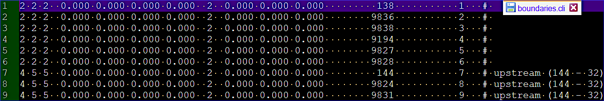
Fig. 122 The boundaries.cli file used in this tutorial starts with the upstream boundary defined in line 7. To find the downstream boundary scroll down to line 313.#
Liquid boundary conditions may be assigned to any open boundary in the *.cli file.
External files instead of PRESCRIBED-keywords
Instead of a list of semi-colon separated numbers in the steering file, liquid boundary conditions can also be defined with a liquid boundary condition file in ASCII text format. For this purpose, the LIQUID BOUNDARIES FILE and/or STAGE-DISCHARGE CURVES FILE keywords need to be defined in the steering file. External files are required for the simulation of quasi-unsteady flows (e.g., a flood hydrograph or low flow sequences for habitat conditions) and more details can be found in sections 4.2.5 and 4.2.6 in the Telemac2d manual or the unsteady section in this eBook.
A velocity profile type can be assigned to any prescribed Q (flowrate) or prescribed U (velocity) open boundary in the form of a list that has the same element order as the above-defined PRESCRIBED … keywords. For this purpose, upstream and downstream velocity profiles can be defined with the VELOCITY PROFILES keyword that accepts the following values:
1is the default option that defines the flow velocity direction at the boundary nodes normal to their edges. This option assigns a length of 1 to the vector and multiplies it with a numeric factor to yield a target flowrate.2reads U and V velocity profiles from the boundary conditions (*.cli) file, which are multiplied with a constant to yield a target flowrate.3imposes the velocity vector direction normal to the boundary and reads the value (UBOR) from the*.clifile, which is then multiplied by a constant to yield a target flowrate.4imposes the velocity vector direction normal to the boundary and calculates the value’s norm proportional to the square root of the water depth. This option can only be used with a prescribed Q open boundary.5imposes the velocity vector direction normal to the boundary and calculates the value’s norm proportional to the square root of a virtual water depth.
With the upstream boundary being a prescribed Q boundary, this tutorial uses VELOCITY PROFILES : 4;1 in the steering file. Read more about options for defining velocity profiles in section 4.2.8 of the Telemac2d manual.
Boundary conditions and mass balance
The boundary condition settings affect mass balance, which is a crucial criterion for a sound numerical model. Read more in the spotlight focus on setting up boundary conditions for mass balance.
Initial Conditions#
The following descriptions refer to section 4.1 in the Telemac2d manual.
The initial conditions describe the state of the model at the beginning of a simulation. Telemac2d recognizes the following types of initial conditions, which can be defined in the steering file with the keyword INITIAL CONDITIONS : 'TYPE' where TYPE can be one of the following:
ZERO ELEVATIONinitializes the free surface elevation at 0 (default). Thus, the initial water depths correspond to the bottom elevation.CONSTANT ELEVATIONinitializes the free surface elevation at a value defined with an INITIAL ELEVATION keyword that has a default value of0.. Thus, the initial water depths correspond to the subtraction of the bottom elevation from the water surface elevation \(wse\). The initial water depth is set to zero at nodes where the bottom elevation is higher than defined by the INITIAL ELEVATION keyword.ZERO DEPTHinitializes the simulation with0(i.e., \(wse\) corresponds to bottom elevation). Thus, the model starts with dry conditions, similar as in the BASEMENT tutorial.CONSTANT DEPTHinitializes the water depths at a value defined by an INITIAL DEPTH keyword that has a default value of0..TPXO SATELLITE ALTIMETRYinitializes the model using information provided by a user-defined database (e.g., the OSU TPXO model for ocean tides). Read more in section 4.2.12 of the Telemac2d manual on modeling marine systems.
To begin, define the initial water depth as 0 with the following keyword, which means that the model will be initialized with a dry riverbed:
INITIAL CONDITIONS : 'ZERO DEPTH'
The simulation speed can be significantly increased when the model has already been running once at the same (initial) discharge. The result of an earlier simulation can be used for the initial condition with the COMPUTATION CONTINUED : YES (default is NO) and PREVIOUS COMPUTATION FILE : *.slf (provide the name of a *.slf file) keywords. This type of model initialization is also referred to as hotstart. Read more about hotstarts in the unsteady simulation and Gaia sections. Also section 4.1.3 in the Telemac2d manual provides descriptions for continuing (hotstart) calculations.
Wet the model at the beginning
Use a constant water depth initial condition of 1 (integer) to speed up calculations, which corresponds to a completely flooded initial model state (i.e., water volume surplus). However, this type initialization will also place a 1-m thick water layer beyond the riverbanks, where water may not be able to run off. Thus, puddles are likely to form longitudinally along the solid 2 2 2 boundaries.
INITIAL CONDITIONS : 'CONSTANT DEPTH'
INITIAL DEPTH : 1
In the case of delta simulations, an initial condition defined with CONSTANT ELEVATION might be preferably defined at a lake or sea level.
Friction (Roughness)#
The following descriptions of friction parameters refer to section 6.1 in the Telemac2d manual.
The LAW OF BOTTOM FRICTION keyword defines a friction law for topographic boundaries, which can be set to:
0for no friction.1for the Haaland [Haa83] equation, which is an implicit form of the Colebrook and White [CW37] equation that builds on the Darcy-Weisbach friction factor \(f_D\). This law involves a high degree of uncertainty that stems from the experimental dataset of the original author.2for the Chézy [Che76] roughness that can be similarly used as3and4.3for Strickler [Str23] roughness \(k_{st}\) (read more, for example, in the 1d hydraulics exercise), which is the inverse of \(n_m\) (4).4for Manning [Man91] roughness \(n_m\) (read more, for example, in the 1d hydraulics exercise), which is the inverse of \(k_{st}\) (3).5for the Nikuradse [Nik33] roughness law, which should correspond to 3 \(\cdot D_{90}\) according to van Rijn [vR19].6for the logarithmic law of the wall for turbulent flows. This option assumes that the average flow velocity is a logarithmic function of the distance from the wall beyond the viscous and buffer layers. The thickness of these layers is a function of the wall roughness length [VK30].7for the Colebrook and White [CW37] equation that calculates the Darcy-Weisbach friction factor \(f_D\) for turbulent flows in smooth pipes.
With respect to the 2d applications in this eBook, the most relevant bottom friction laws are 3 [Str23], 4 [Man91], and 6 (log law). The Nikuradse [Nik33] roughness law (5) is recommended for 3d simulations (see the Telemac3d tutorial). Friction is more generally referred to as with the general coefficient \(c_{f}\), which has a particular relevance for bedload transport (cf. morphodynamic calculations with Gaia).
The FRICTION COEFFICIENT FOR THE BOTTOM keyword sets the value for a characteristic roughness coefficient. For instance, when the friction law keyword is set to 3 [Str23], the friction corresponds to the Strickler roughness coefficient \(k_{st}\) (in fictive units of m\(^{1/3}\) s\(^{-1}\)). For rough channels (e.g., mountain rivers) \(k_{st} \approx 20\) m\(^{1/3}\) s\(^{-1}\) and for smooth concrete-lined channels \(k_{st} \approx 75\) m\(^{1/3}\) s\(^{-1}\). In fully turbulent flows, the Strickler roughness can be approximated with \(k_{st} \approx \frac{26}{D_{90}^{1/6}}\) [MPM48] where \(D_{90}\) is the grain diameter of which 90% of the surface grain mixture are finer.
This tutorial features the application of a Manning roughness coefficient of \(n_m\)= 0.03, which is the inverse of \(k_{st}\) and implemented with:
LAW OF BOTTOM FRICTION : 4 / 4-Manning
FRICTION COEFFICIENT : 0.03 / Roughness coefficient
Expand to see exemplary values for Manning roughness
Table 8 lists exemplary values for the Manning roughness coefficient \(n_m\) based on Aldridge and Garrett [AG73] and Arcement and Schneider [AS89].
Surface type |
Material diameter (10\(^{-3}\)m) |
\(n_m\) (m\(^{-1/3}\)s) |
|---|---|---|
Concrete |
\(-\) |
0.012-0.018 |
Firm soil |
\(-\) |
0.025-0.032 |
Coarse sand |
1-2 |
0.026-0.035 |
Gravel |
2-64 |
0.028-0.035 |
Cobble |
64-256 |
0.030-0.050 |
Boulder |
\(>\) 256 |
0.040-0.070 |
Friction zones (regional friction values)
To create zones with different friction values, have a look at the spotlight focus on roughness zones.
In addition, specific roughness conditions should be defined for the liquid boundaries (see above), which should not be changed in the process of model calibration later. To this end, a measured stage-discharge relation is required to back-calculate cross-section averaged hydraulics. For this purpose, take a look at the Python exercise on 1-d hydraulics for solving the Manning-Strickler formula.
LAW OF FRICTION ON LATERAL BOUNDARIES : 3 / integer (3 is Strickler)
ROUGHNESS COEFFICIENT OF BOUNDARIES : 33.3 / float inverse of n_m=0.03
Differentiate between bottom and boundary friction
Not using the two keywords defining the friction at the boundaries will make that any roughness calibration affects the mass balance.
Turbulence#
The following descriptions refer to section 6.2 in the Telemac2d manual.
Turbulence describes a seemingly random and chaotic state of fluid motion in the form of three-dimensional vortices (eddies). True turbulence is only present in 3d vorticity and when it occurs, it mostly dominates all other flow phenomena through increases in energy dissipation, drag, heat transfer, and mixing [KC08]. The phenomenon of turbulence has been a mystery to science for a long time, since turbulent flows (read more about the implementation in RANS) have been observed, but could not be explained by the linear equations systems. Today, turbulence is considered a random phenomenon that can be accounted for in linear equations, for instance, by introducing statistical parameters. For instance, when turbulence applies to the depth-averaged Navier-Stokes equations a numerical solution for a quantity (e.g., flow velocity) corresponds to \(value = \overline{mean value} + value fluctuation'\). For this purpose, there are a variety of options for implementing turbulence in numerical models [NN93].
The horizontal and vertical dimensions of turbulent eddies can vary greatly, especially in rivers and transitions to backwater zones (tidal flats) where the wide horizontal flow dimension (river width \(w\)) is significantly larger than the vertical flow dimension (water depth \(h\)): \(w >> h\). Telemac2d provides multiple turbulence models that can be applied to the vertical and/or horizontal dimensions and defined with the TURBULENCE MODEL keyword being an integer number for one of the following options:
1to use a constant viscosity coefficient (default) for turbulent viscosity, molecular viscosity, and Diffusion. This closure option should not be used with Stage-discharge relation open boundaries (i.e., do not use with prescribed Q and H) [WBH02].2to use the Elder formula for the Diffusion coefficient \(D\). The Elder turbulence closure also yields small errors for Stage-discharge relation open boundaries (i.e., do not use this option with prescribed Q and H) [WBH02].3to use the \(k-\epsilon\) two-equation model solving the Navier-Stokes equations. The first equation represents a turbulence closure for the turbulent kinetic energy \(k\); the second equation is a turbulence closure for the turbulent dissipation \(\epsilon\). Both equations express that the sum of change of (I) \(k\) and \(\epsilon\) in time, and (II) Advection transport of \(k\) and \(\epsilon\) equal the sum of (1) Diffusion transport of \(k\) and \(\epsilon\), (2) the production rate of \(k\)/\(\epsilon\), and (3) the destruction rate of \(k\)/\(\epsilon\) [LS74]. The \(k-\epsilon\) model is a generalization of the mixing length model (see option5) and assumes that the turbulent viscosity is isotropic (valid for many river applications, but not for circular-rotating flows or groundwater) [Bra87]. Thus, the \(k-\epsilon\) model introduces two additional equations and requires a finer mesh than the constant viscosity option1, which leads to a longer computation time. Yet, the \(k-\epsilon\) model generally yields accurate results and small errors with Stage-discharge relation open boundaries [WBH02]. The following default keywords are associated with the \(k-\epsilon\) model:VELOCITY DIFFUSIVITY : 1.E-6corresponding to the kinematic viscosity \(\nu\) of water (10\(^{-6}\) m\(^2\)/s).TURBULENCE REGIME FOR SOLID BOUNDARIES : 2for rough walls of closed boundaries to apply the value chosen for the LAW OF BOTTOM FRICTION and ROUGHNESS COEFFICIENT OF BOUNDARIES keywords (recall section Friction (Roughness)). For smooth closed boundary walls setTURBULENCE REGIME FOR SOLID BOUNDARIES : 1.INFORMATION ABOUT K-EPSILON MODEL : YESenables console output of information on the \(k-\epsilon\) closure solution.
4to use the Smagorinsky [Sma63] (also known as general circulation) model, which stems from climate modeling. It represents a large eddy simulation (LES, in contrast to RANS). The Smagorinsky [Sma63] model does not account for Diffusion.5to use a mixing length model according to Prandtl’s theory that a fluid quantity conserves its properties for a characteristic length before it mixes with the bulk flow [Bra74].6to use the Spalart and Allmaras [SA92] model that solves the continuity equation for a viscosity-like, kinematic eddy turbulent viscosity. The Spalart and Allmaras [SA92] model was originally developed for aerodynamic flows with low Reynolds number. It represent a detached eddy simulation (DES, in contrast to RANS).
This tutorial uses the \(k-\epsilon\) model (3) because of its popularity and wide applicability (not to confuse with correctness).
DIFFUSION OF VELOCITY : YES / enabled by default
TURBULENCE MODEL : 3
Run Telemac2d#
With the steering (*.cas) file, the last necessary ingredient for running a steady hydrodynamic 2d simulation with Telemac2d is available. Make sure to put all required files in one simulation folder (e.g., ~HOMETEL/mysimulations/steady2d-tutorial/). The required files can also be downloaded from this eBook’s steady2d tutorial repository and include:
With these files prepared, load the TELEMAC environment, and run Telemac2d following the explanations in the next sections.
Load environment and files#
Go to the configuration folder of the Telemac installation (e.g., HOMETEL/configs/ where HOMETEL could be something like /home/telemac/v9.0.0/) and load the environment (e.g., pysource.gfortranHPC.sh - use the same as for compiling Telemac).
cd ~/telemac/v9.0.0/configs
source pysource.gfortranHPC.sh
If you are using the Hydro-Informatics (Hyfo) Mint VM
If you are working with the Mint Hyfo VM, load the TELEMAC environment as follows:
cd ~/telemac/v8p2/configs
source pysource.hyfo-dyn.sh
Start a Telemac2d simulation#
To start a simulation, change to the directory (cd) where the simulation files live and run the steering file (.cas) with the telemac2d.py script:
cd ~/telemac/v9.0.0/mysimulations/steady2d-tutorial/
telemac2d.py steady2d.cas -s
The -s flag is not strictly needed but useful for revising simulation characteristics, such as fluxes across the liquid boundaries or the total simulation time. It will write a file named steady2d.cas.[...].sortie and can be used for convergence analysis described in the spotlight chapter on quantitative convergence.
As a result, a successful computation should end with the following lines (or similar) in Terminal:
[...]
                     *************************************
                     *    END OF MEMORY ORGANIZATION:    *
                     *************************************

 CORRECT END OF RUN

 ELAPSE TIME :
                             03  MINUTES
                             44  SECONDS
... merging separated result files

... handling result files
        moving: r2dsteady.slf
... deleting working dir

My work is done
Thus, Telemac2d produced the file r2dsteady.slf that can now be analyzed in the post-processing with QGIS or ParaView.
Post-processing#
The post-processing of the steady 2d scenario uses QGIS and the PostTelemac plugin. Alternatively, Telemac results can also be visualized with ParaView or BlueKenue.
Load results and the Q4TS Plugin#
Launch QGIS, create a new QGIS project, set the project CRS to UTM zone 33N, add a satellite imagery basemap, and save the project (e.g., as tm2d-postpro.qgis) in the same folder where the Telemac2d simulation results file (r2dsteady.slf is located), similar to the descriptions in the pre-processing tutorial.
Load the r2dsteady.slf geometry file as mesh layer with drag and drop from the Browser panel to the Layers panel. Make sure to import it with its correct georeference: EPSG:32633 (ETRS 89 / UTM zone 33N).
To continue with this section, make sure the Q4TS plugin is installed (see instructions in the Software Requirements section <qgis-telemac>). To explore results without the Q4TS plugin, directly jump to the next section <tm2d-post-export. Q4TS is helpful to perform SALOME/ParaVis-like analysis (e.g., advanced probing, post-processing pipelines, MED-centric workflows) through conversion processing:
In Processing > Toolbox, run slf2med (Q4TS provider):
Input .slf:
r2dsteady.slfInput .cli (optional): your boundary file if you want it carried along
Output .med: save
r2dsteady.med
Then open the *.med file in your preferred MED-capable post-processing workflow (ParaVis/SALOME). This is the one Q4TS feature that meaningfully bridges into “real post-processing” outside QGIS.
Cross-section analysis (extract values along section lines)#
This replaces the old “draw a line and inspect/export” routine from PostTelemac, but it’s cleaner because it produces a reproducible CSV from a line layer.
Create a cross-section line layer:
Create a new line layer (GeoPackage recommended) called, for example,
control_sections.Digitize one or multiple cross-section lines across the channel (upstream, downstream, control sections, etc.).
Export cross-section values from the mesh to CSV
Open Processing > Toolbox and run Export cross section dataset values on lines from mesh
Configure:
Input mesh layer:
r2dsteadyDataset groups: choose what you want to analyze (examples)
WATER DEPTH(stability / wetting-drying behavior)velocity components or magnitude (hydraulics + stability hotspots)
any diagnostic variable you wrote to the results (if available)
Dataset time:
use Current canvas time for “snapshot” checks, or
run multiple times for specific timestamps you care about.
Lines for data export:
control_sectionsLine segmentation resolution: set this to something that makes sense for your mesh resolution (don’t oversample).
Output: save as
*.csv
Open the exported CSV in Libre Office and plot section profiles (e.g., depth vs. chainage, velocity vs. chainage). Repeat for upstream/downstream sections and compare.
What this tells you (model performance angle):
section-by-section sanity checks (e.g., depth/velocity patterns where you expect them),
hotspot detection (unphysical spikes near boundaries, around steep bathymetry gradients, etc.),
“is it steady yet?” checks by comparing the same section at multiple timesteps.
Node analysis (time series at control points)#
For convergence / stability checks, point time series are usually the fastest signal.
Create a control-point layer:
Create a point layer called
control_points.Add points at locations you care about:
near inflow/outflow boundaries,
near hydraulic controls,
in zones where instability is likely (shallow areas, strong gradients, wetting/drying front).
Export time series from the mesh to CSV:
Open Processing > Toolbox and run Export time series values from points of a mesh dataset
Configure:
Input mesh layer:
r2dsteadyDataset groups: pick the key variables you want to monitor (depth, velocity, and any diagnostic fields you output)
Points for data export:
control_pointsOutput: save as
*.csv
Plot the time series in Libre Office and use it as a quick performance dashboard:
Does depth/velocity settle to a stable value (steady state)?
Do you see oscillations or spikes (numerical issues, boundary-condition problems)?
Do shallow nodes flip wet/dry unrealistically (wetting/drying tuning issue)?
These extracted series are directly usable in the wet initialization exercise below.
Export to GeoTIFF#
To export the model results to a GeoTIFF raster, go to the Processing Toolbox (in QGIS), expand the Mesh entry, and open the Rasterize mesh dataset tool. In the Rasterize Mesh Dataset popup window (Figure 123) make the following settings:
Input mesh layer: select the Telemac results mesh layer (
r2dsteady)Dataset groups: click on the … button > Select in Available Dataset Groups and select a quantity of interest. This tutorial features the export of a flow velocity. Click OK to return to the Rasterize Mesh Dataset tool.
Dataset time: click on the up/down arrow symbol to scroll to the bottom and select the last timestep. In an unsteady (i.e., quasi-steady) simulation, other timesteps might be of interest, too.
Extent: click on the dropdown arrow > Calculate from Layer > select r2dsteady
Pixel size:
1.0(default). With coarser or finer meshes, the pixel size should be varied.Output coordinate system: select
EPSG:32633(that is, the coordinate reference system of the mesh)Output raster layer: click on … to navigate to a target folder and enter a name for the raster. Here:
velocity-tmax.tif.Run the rasterization.
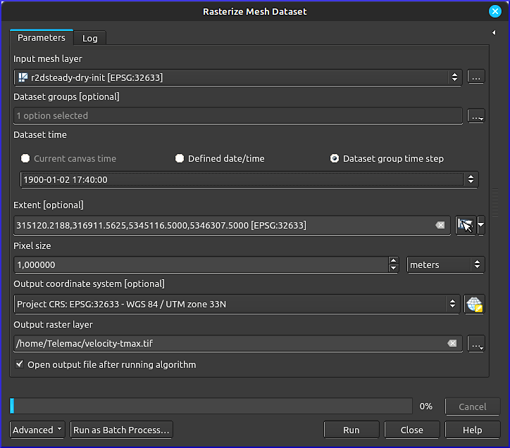
Fig. 123 The Rasterize Mesh Dataset tool in QGIS.#
The resulting velocity-tmax raster will be added to the Layers panel. For better visualization, some color is helpful. Therefore, double-click on the new velocity-tmax to open its properties. Go to the Symbology, change the Render type to Singleband pseudocolor, and use your favorite color ramp and number of classes for visualizing the velocity. To make 0-entries invisible, click on their Color symbol and set the Opacity to 0%, or set the Min to 0.0001.
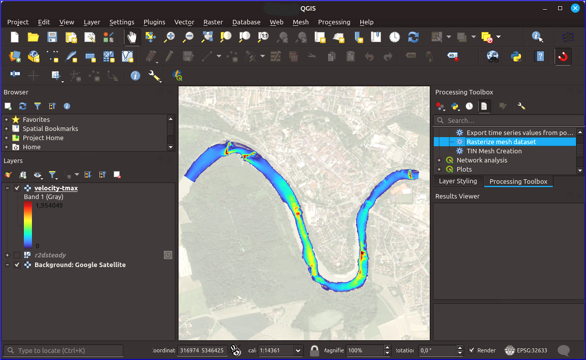
Fig. 124 The exported flow velocity (VITESSE) GeoTIFF raster in QGIS (background map: Google [Goond] satellite imagery). The location of the Raster mesh dataset tool in the Processing Toolbox is highlighted on the right.#
Analyze Results#
The first analysis of results should address the basic correctness of the model, for instance, regarding mass balance and its evolution over time. For this purpose, open the Time Controller  in QGIS top menu.
Quantitative Discharge Convergence#
During the simulation, the keywords MASS-BALANCE : YES and/or PRINTING CUMULATED FLOWRATES : YES print mass fluxes across liquid boundaries in the Terminal. To retrospectively review flux rates and volume balance, the simulation must have run with the -s flag, which saves the simulation state in a file called similar to steady2d.cas_YEAR-MM-DD-HHhMMminSSs.sortie. Based on the .sortie file, sums of fluxes, the total volume, and volume error can be extracted and analyzed with the Python scripts provided along with the Telemac installation (HOMETEL/scripts/python3/). The Telemac Jupyter notebooks (HOMETEL/notebooks/ > data_manip/extraction/*.ipynb or workshops/exo_fluxes.ipynb) exemplify the usage of the Python scripts. A detailed discussion on convergence and tweaked Python scripts (pythomac) can be found in this eBook, in the chapter on quantitative Telemac convergence analysis. With these scripts, Fig. 125 was generated showing the flows across the two boundaries of the steady-2d study, indicating convergence after approximately 7000 timesteps.

Fig. 125 Flux convergence plot across the two boundaries of the dry-initialized steady Telemac2d simulation (created with pythomac).#
Qualitative Velocity, Depth, and Discharge Evolution#
The convergence of water depth and flow velocity, and therefore, discharge, can be qualitatively observed in QGIS through the Time Controller (see activation in Fig. 126). The frequency of images can be set through clicking on the cogwheel of the time controller, and image sequences played by clicking in the Play button. Additionally, Fig. 126 uses an overlay of water depth pixel colors (contour plot), and flow velocity vectors, defined in the Layer Styling panel. The North and discharge arrows, and the title are Decorators, which can be found in View > Decorators.
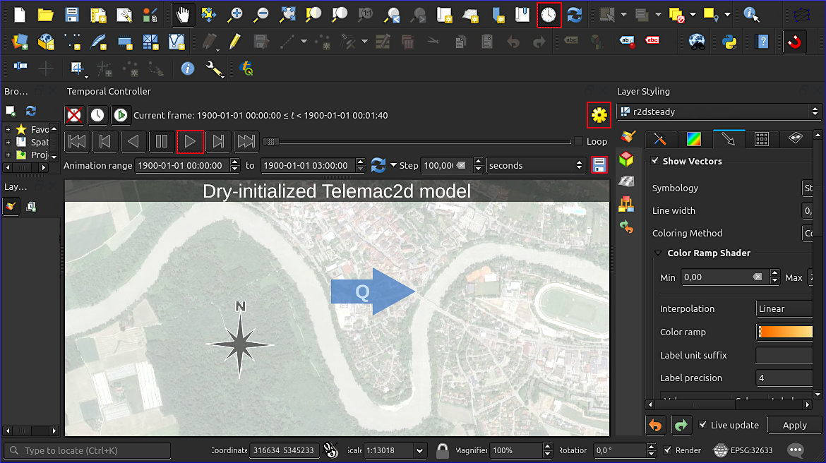
Fig. 126 The activated time controller in QGIS enables to move along the time axis of modeled quantities (background map: Google [Goond] satellite imagery). The red-highlighted buttons activate the time controller, play the sequence of images of selected quantities, provide a setting for playing a frequency of images per second, and enable saving images of all timesteps (see instructions below).#
To export a series of images for turning them into a movie-like GIF, use the Save button of the time controller. Set up the desired resolution and define an output folder. The series of PNG images can then be converted, for example, with GIMP, into a GIF. For this purpose, download and open GIMP, then:
Open the first image of the exported series.
Pull all other exported images into the Layers panel of GIMP.
Reverse the order of the layers in GIMP: Layer > Stack > Reverse Layer Order.
Save the image as GIF: File > Export As….
Select a folder to save the file, in the Name field enter
[any-name].GIF, and click Export.In the popup window enable As animation and Loop forever with a recommended delay between frames of 100 milliseconds. Keep all other defaults and click Export.
The animated figure below features an exported GIF with water depth in the background and flow velocity as streamline-vectors ranging from 0 to 2.0 m/s. The animation shows how the model is filled from both its upstream (left) and downstream (right) boundaries at the beginning of the simulation. While the upstream discharge was imposed along with a water depth through a 5 5 5 boundary, the downstream boundary only had a prescribed water depth 5 4 4 boundary. The prescription of sufficient water depths was necessary to avoid supercritical flows at the boundaries, which would make the numerical model crash immediately. Because the flux coming from the downstream boundary needs to move uphill, it cannot go very fast and is rolled over by a wave of water coming from the upstream boundary. If a downstream flux was prescribed, the model would have been more unstable and overdetermined.
GIF sequence of a dry-initialized Telemac2d model (large file size!)
Recall: boundary conditions and mass balance
Mass balance is a crucial criterion for a sound numerical model. Read more in the spotlight chapter on setting up boundary conditions for mass balance.
Exercise: Initial Conditions#
The above Fig. 197 and depth-velocity animation point to stability achieved after approximately 7000 timesteps. A wet-initialized model converges much faster, but either requires a previous run of a dry model initialization, or it can make use of other initial condition keywords in Telemac. Ideally, the dry-initialized model is used as a so-called hotstart condition for a wet-initialized model, as described in the unsteady 2d tutorial.
Challenge: initialize Telemac with an initial water depth
Even though it is not best practice for modeling a river, running the steady2d.cas simulation with an initial water depth of 1 m is an interesting exercise to experience why it is not a good choice. To run the model with an initial water depth, we can facilitate the boundary conditions by removing the upstream depth constraint (i.e., setting the first entry of the PRESCRIBED ELEVATIONS keyword to 0.), and modifying the INITIAL [...] condition keywords to a 'CONSTANT DEPTH' of 1 meter:
/ steady2d_wet.cas
/ ... header
/ ...
PRESCRIBED FLOWRATES  : 35.;0.
PRESCRIBED ELEVATIONS : 0.;371.33
/ ...
INITIAL CONDITIONS : 'CONSTANT DEPTH'
INITIAL DEPTH : 1
/ ...
/ ... footer
Also, change the upstream boundary type to a less constrained 4 5 5 (prescribed Q only) type in the boundaries.cli file. For this modification, it is sufficient to open boundaries.cli in any text editor and use its find-and-replace function (e.g., CTRL + H keys in NotepadPlusPlus (Text Editor)):
In the Find field type
5 5 5.In the Replace with field type
4 5 5.Click on Replace until all upstream boundary node types are modified.
Save and close boundaries.cli.
Save the modified .cas and .cli files, and re-run Telemac:
telemac2d.py steady2d_wet.cas
The diagram in Fig. 127 plots the two columns of flows at the upstream and downstream open boundaries over time for the simulation setup in this tutorial. The diagram suggests that the model reaches stability (i.e., converges) after the 55th output listing (simulation time \(t \leq 5500\)).
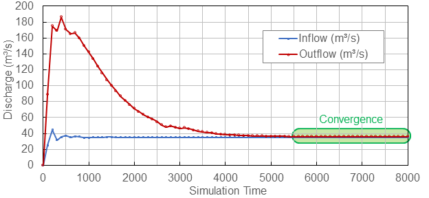
Fig. 127 Convergence of inflow (upstream) and outflow (downstream) at the open model boundaries of a wet model.#
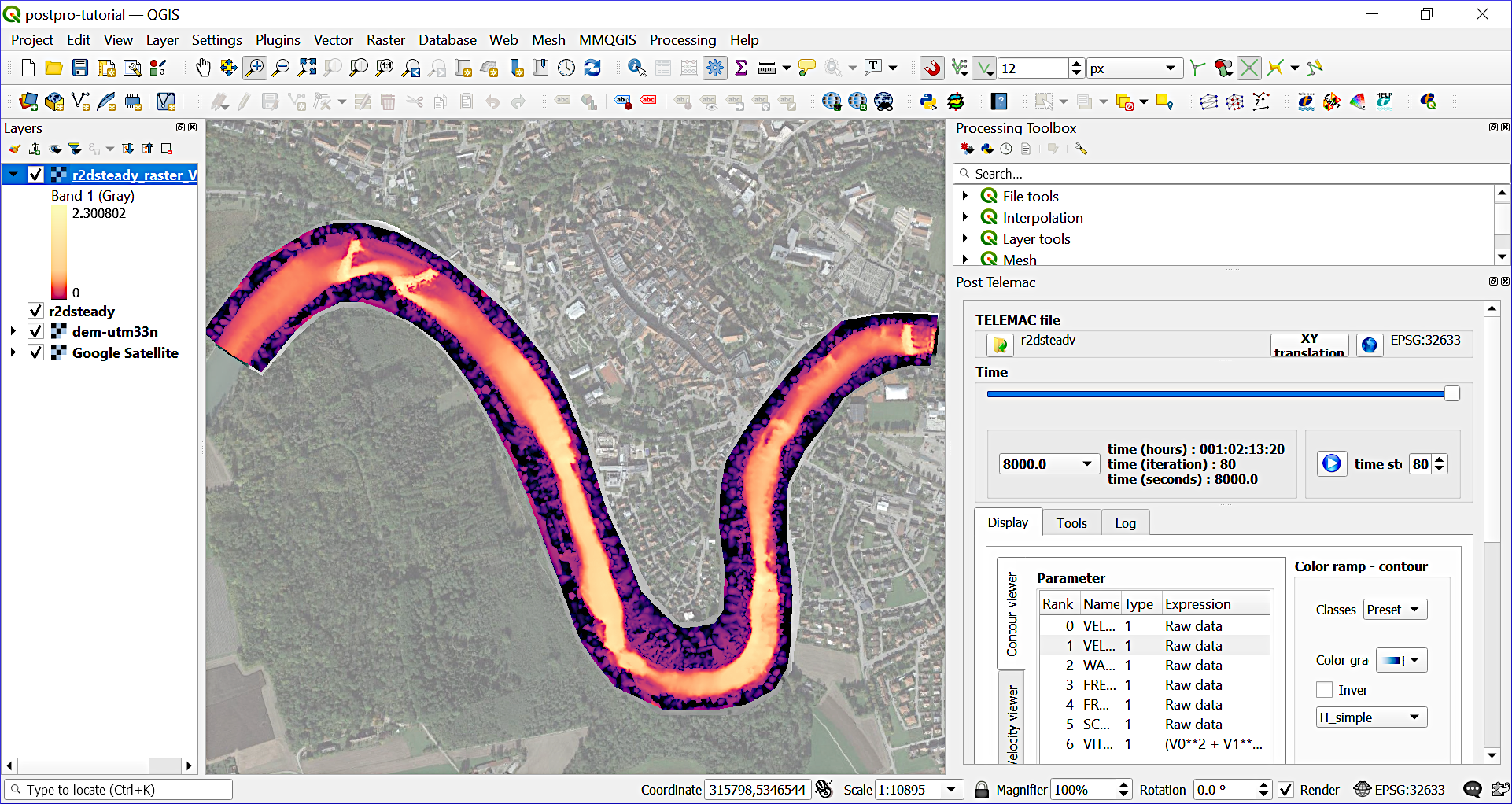
Fig. 128 The flow velocity (VITESSE) GeoTIFF raster after a wet-initialized Telemac simulation, shown in QGIS (background map: Google [Goond] satellite imagery).#
Question: what are the pros and cons of the wet-initialized simulation with constant water depth?
Positive (pro) is that the simulation converges considerably faster than in the case of the dry-initialized model.
Negative (contra) performance indicators are some non-zero flow velocity pixels on the floodplains (beyond the riverbanks) in Fig. 128. These apparently wrongly modeled pixels are an artifact of the use of wet initial conditions, which put a 1-m thick water layer all over the model. Specifically, water patches remained in small, local terrain depressions between the solid boundaries (2 2 2) and dykes along the riverbanks. This water could not run off and stayed on these patches until the end of the simulation. This is a physically unreasonable no-go flag, which disqualifies a model for any application.
Notes on Calibration#
Refresher: How does calibration work?#
Calibration involves the step-wise adaptation of model input parameters to yield a possibly best (statistic) fit of modeled and measured data. In the process of model calibration, only one parameter should be modified at a time by 10 to 20-% deviations from its default value. For instance, if the beginning FRICTION COEFFICIENT : 0.03, the calibration may test for FRICTION COEFFICIENT : 0.033, then FRICTION COEFFICIENT : 0.036, FRICTION COEFFICIENT : 0.027 and so on, ultimately to find out which value for FRICTION COEFFICIENT brings the model results closest to observations.
Moreover, a sensitivity analysis compares step-wise modifications of multiple parameters (still: one at a time) and theirs effect on model results. For instance, if a 10-% variation of FRICTION COEFFICIENT yields a 5-% change in global water depth while a 10-% variation of grid size (edge length) yields a 20-% change in global water depth, it may be concluded that the model sensitivity is higher with respect to the grid size. However, such conclusions require careful considerations in multi-parametric, complex models of river ecosystems.
Calibration Parameters in Telemac#
The following parameters may be used for calibrating a 2d model to measurements (e.g., water surface elevation, water depth, or flow velocity data):
FRICTION COEFFICIENT (friction section)
Solvers, solver options, implicitation and other numerical parameters (numerical parameter section)
Type of model initialization
Avoid accuracy-reducing keyword settings
Keyword settings such as MASS-LUMPING ... : ... lead to increased smoothing (i.e., reduced accuracy) of results to increase computation speed. However, in most cases, it is worth accepting longer computation times and yielding higher accuracy, which will reduce efforts for model calibration, and thus, saves more time in the end.
Next Steps#
Make sure the simulation is conservative according to the descriptions in the spotlight chapter on mass balance.
Find a meaningful simulation duration for convergence of a dry-initialized simulation following the algorithms provided with the chapter on quantitative convergence.
Use the dry-initialized model to simulate at least 2-3 steady discharges (with hotstart conditions) for which measurement data is available for calibration and validation.
The calibrated and validated model can be
used for unsteady hydrodynamic simulations, and
serve a basis for morphodynamic sediment transport modeling with Gaia.