Pre-processing

Requirements

This tutorial is designed for advanced beginners and before diving into this tutorial make sure to:

• Follow the installation instructions for QGIS in this eBook.

• Read (or watch) and understand this eBook’s QGIS Tutorial.

• Install BlueKenue.

The first steps in numerical modeling of a river with TELEMAC consist in the conversion of a Digital Elevation Model (DEM) into a computational mesh. This tutorial guides through the creation of:

• A QGIS project for creating a computational mesh (similar to the BASEMENT pre-processing).

• Optionally, the mesh generation with the BlueKenue^TM software is featured.

• A BlueKenue workspace to interpolate terrain elevations from a DEM, including the export of a mesh to the SELAFIN/SERAFIN (.slf) geometry format for Telemac, and the definition boundary edges.

At the end of this tutorial, TELEMAC users will have generated a computational mesh in the *.slf file format, which is ready to use for the Telemac2d steady simulation tutorial. Additional materials and intermediate data products are provided in this eBook’s supplemental telemac data repository.

Platform compatibility

All software applications featured in this tutorial can be run on Linux, Windows, and also potentially macOS (not tested) platforms.

QGIS

Create and Setup a New Project

Launch QGIS and create a new QGIS project to get started with this tutorial. As featured in the QGIS Tutorial, set up a coordinate reference system (CRS) for the project. This example uses data of a river in Bavaria (Germany, UTM zone 33N), which requires the following CRS:

• In the QGIS top menu go to Project > Properties.

• Activate the CRS tab.

• Enter UTM zone 33N and select the CRS shown in Fig. 101: EPSG 32633.

• Click Apply and OK.

Note that the CRS used with TELEMAC differs from the one used with BASEMENT to enable the compatibility of geospatial data products from QGIS with BlueKenue. Also, EPSG 32633 is not a great choice because of its low precision (at best 2 m), but it will do the job for this tutorial.

Fig. 101 Define UTM zone 33N (WGS84) as project CRS.

Save the project…

Save the QGIS project (Project > Save As…), for example, with the name prepro-tutorial.qgz.

Third-party Plugins

The TELEMAC tutorials rely on the BASEmesh plugin and the PostTelemac plugin. To this end, open the QGIS plugin manager (Plugins menu > Manage and Install Plugins) to open the Plugins window (Fig. 102).

Fig. 102 Open QGIS’ Plugins Manager.

In the Plugins window, add both plugins as follows:

• BASEmesh requires to add the developer’s plugin repository (more details are available in the BASEMENT pre-processing tutorial):

  • Go to the Settings tab.

  • Scroll to the bottom (Plugin Repositories listbox in Fig. 69), click on Add….

  • In the popup window enter:

    • a name for the new repository, for instance, BASEmesh Plugin Repository;

    • the repository address: https://people.ee.ethz.ch/~basement/qgis_plugins/qgis_plugins.xml.

  • Click OK. The new repository should now be visible in the Plugin Repositories listbox.

• Install the BASEmesh plugin:

  • Go to the All tab (still in the Plugins window) and enter basemesh in the search field.

  • Find the newest BASEmesh (i.e., Available version >= 2.0.0) plugin and click on Install Plugin.

• To install the PostTelemac plugin type posttelemac in the All tab and click on Install Plugin.

• After the successful installation Close the Plugins window.

Now, the BASEmesh 2 plugin should be available in QGIS’ Plugins menu and the PostTelemac symbol should be visible in QGIS’ menu bar.

Why use BASEmesh for TELEMAC?

By using BASEmesh, this tutorial employs BASEMENT’s efficient mesh generator to minimize the number of work steps to be made in BlueKenue^TM. The rationale behind this approach is that QGIS is more stable and user-friendly than BlueKenue^TM, for instance, to correct drawing errors of boundary lines.

Load DEM

This tutorial uses height information that is stored in a DEM. For the QGIS section, preferably use the GeoTIFF DEM with UTM zone 33N as CRS as follows:

• Download the GeoTIFF DEM and save it in the same folder (/ProjectHome/ or a sub-directory) as the above-create qgz project.

• Add the downloaded DEM as a new raster layer in QGIS:

  • In QGIS’ Browser panel find the ProjectHome directory where you downloaded the DEM tif.

  • Drag the DEM tif from the ProjectHome folder into QGIS’ Layer panel.

• To facilitate delineating specific regions of the river ecosystem later, add a satellite imagery basemap (XYZ tile) under the DEM and customize the layer symbology.

What are QGIS panels, what is a basemap, and how can I re-order layers?

Learn more in the QGIS tutorial on Panels, Toolbars, and Plugins.

The dem-utm33n layer should now be visible in the viewport and listed in the Layers panel. Right-click on the dem-utm33n layer and select Zoom to Layer(s) to view the layer.

Alternatively work with a .xyz DEM pointcloud

This tutorial uses later in the section on BlueKenue^TM a *.xyz file as DEM, which was derived from the GeoTIFF using the workflow described in the QGIS tutorial. The *.xyz file can also be used with QGIS and it can be downloaded here. To import the dem.xyz file in QGIS, open the Data Source Manager from the Layer top menu, select Add Layer and Add Delimited Text Layer…. In the opening Data Source Manager window (see Fig. 103) take the following actions:

• Select the downloaded dem.xyz file in the file name field.

• In the File Format frame, make sure to select Custom delimiters and check the Space delimiter box.

• In the Record and Fields Options frame, set the Number of header lines to discard to 13 and check the First record has field names box.

• In the Geometry Definition frame, select :EndHeader as X field, field_2 as Y field, and field_3 as Z field. Select Project CRS: ESRI:32633 - WGS 84 / UTM zone 33N as Geometry CRS.

• Click Add and Close the Data Source Manager window.

Fig. 103 Import the *.xyz point cloud as QGIS layer.

Enable Snapping

It is important that the lines do not overlap to avoid ambiguous or missing definitions of regions and to ensure that boundary lines are closed. Therefore, activate snapping:

• Activate the Snapping Toolbar: View > Toolbars > Snapping Toolbar

• In the Snapping toolbar > Enable Snapping

• Enable snapping for

  • Vertex, Segment, and Middle of Segments .

  • Snapping on Intersections .

  • Self Snapping .

Model Boundaries and Breaklines

This section resembles the instructions of the BASEMENT pre-processing tutorial to generate an SMS 2dm mesh file. The differences are that the shapefiles for the TELEMAC pre-processing use the UTM zone 33N CRS and that the height (elevation) interpolation needs to be done with the BlueKenue^TM software to generate liquid boundary lines and an *.slf geometry file for TELEMAC. The generation of the SMS 2dm mesh relies on the QGIS BASEmesh plugin and requires drawing a

• Line Shapefile called breaklines.shp that contains model boundaries and internal breaklines between model regions with different characteristics;

• Line Shapefile called liquid-boundaries.shp that contains model boundaries for assigning inflow and outflow conditions;

• Point Shapefile called region-pts.shp that contains markers for the definition of characteristics of model regions.

Figure 104 provides an overview of the shapefiles to be drawn for generating a quality mesh with the BASEmesh plugin.

Fig. 104 The breaklines, liquid boundaries, and region points shapefile to draw for creating a 2dm quality mesh with the BASEmesh plugin (background map: Google [Goond] satellite imagery).

Breaklines and Model Outline

The model boundary defines the model extent and can be divided into regions with different characteristics (e.g., roughness values) through breaklines. Breaklines indicate, for instance, channel banks and the riverbed (main channel), and need to be inside the DEM extents. Boundary lines and breaklines are stored in a Line Shapefile that BASEmesh uses to find both model boundaries and internal breaklines between model regions. For this purpose, Create a Line Shapefile and call it breaklines.shp (Layer > Create Layer > New Shapefile Layer). Click on QGIS’ Layers menu > Create Layer > New Shapefile Layer… (see Fig. 105). Make sure to select EPSG: 32633 - WGS 84 / UTM zone 33N as CRS . Do not add any field.

Fig. 105 Create a new shapefile from QGIS’ Layers menu.

Start editing breaklines.shp by clicking on the yellow pen and draw the breaklines indicated in Fig. 104 by activating Add Line Feature , which involves:

• The boundaries of the model at the left and the right floodplain limits:

  • Delineate the outer bounds of the floodplains.

  • Make sure that all points and lines are inside the DEM layer.

  • Do not cross the river (wetted area indicated by the satellite imagery basemap).

  • Finalize every line with a right-click.

• The breaklines of the left bank (LB) and right bank (RB):

  • Draw lines along the wetted main channel indicated in the satellite imagery (basemap).

  • Make sure that line ends perfectly coincide with the before-created floodplain boundary lines (snapping is needed); thus, the main channel’s breaklines and the floodplain boundary lines need to enclose the floodplains without any gap between the lines.

• Breaklines of gravel banks:

  • Draw lines along the gravel banks that are visible in the satellite imagery basemap in the main channel.

  • Make sure that the line ends perfectly coincide (use snapping) with the before-created main channel breaklines; thus, the main channel’s hard breaklines and the gravel bank breaklines need to enclose the gravel banks without any gap between the lines.

• Optional: Breaklines of block ramps:

  • Find the rough block ramps (effervescing waters) in the satellite imagery basemap and delineate them by drawing lines across the wetted main channel.

  • Make sure that the line ends perfectly coincide with the main channel breaklines; thus, the main channel’s hard breaklines and the block ramp breaklines need to enclose the block ramps without any gap between the lines.

To correct drawing errors use the Vertex Tool . Finally, save the new lines (edits of breaklines.shp) by clicking on the Save Layer Edits symbol. Stop (Toggle) Editing by clicking again on the yellow pen symbol.

Troubles with drawing boundaries and breaklines?

Download the zipped breaklines shapefile shown in the above figure and unpack it into the project folder, for instance, /ProjectHome/shapefiles/breaklines.[SHP].

Draw boundaries of complex DEMs…

Drawing boundaries manually around large DEMs can be very time consuming, in particular, if the raw data are a point cloud and not yet converted to a Gridded Cell (Raster) Data.

If you are dealing with a point cloud, consider using QGIS Convex Hull tool that draws a tight bounding polygon around points.

If you are dealing with a large GeoTIFF, consider using QGIS’ Raster to Vector tool.

Liquid Boundaries

The liquid boundaries define where hydraulic conditions, such as a given discharge or stage-discharge relationship, apply at the model inflow (upstream) and outflow (downstream) limits. Thus, a functional river model requires at least one inflow boundary (line) where mass fluxes enter the model and one outflow boundary (line) where mass fluxes leave the model. For this purpose, Create a Line Shapefile called liquid-boundaries.shp, select EPSG: 32633 - WGS 84 / UTM zone 33N as CRS , and define two text data fields named type and stringdef. Make sure that snapping is still enabled and Toggle (Start) Editing the new liquid-boundaries.shp. Then draw two lines:

• Activate Add Line Feature .

• Draw an inflow boundary line (light blue line on the left of Fig. 104):

  • Zoom to the inflow region of the DEM limits, where there is a gap between the above-created floodplain boundary breaklines.

  • Start drawing a line on one bank (top of the below figure) and move to the other bank to make approximately seven more points across the river.

  • The last point needs to coincide with the end of the other bank’s floodplain boundary breakline.

  • Finalize the line with a right-click, and enter Inflow in the type field and inflow in the stringdef field (the case matters).

• Draw an outflow boundary line (light blue line on the right of Fig. 104):

  • Zoom to the outflow region of the DEM limits, where there is a gap between the above-created floodplain boundary breaklines.

  • Start drawing a line on one bank (top of the below figure) and move to the other bank to make approximately seven more points across the river.

  • The last point needs to coincide with the end of the other bank’s floodplain boundary breakline.

  • Finalize the line with a right-click, and enter Outflow in the type field and outflow in the stringdef field (the case matters).

To correct drawing errors use the Vertex Tool .

Finally, save the liquid boundary lines (edits of liquid-boundaries.shp) by clicking on the Save Layer Edits symbol. Stop (Toggle) Editing by clicking again on the yellow pen symbol.

Troubles with drawing the liquid boundary lines?

Download the zipped liquid-boundaries shapefile and unpack it into the project folder, for instance, /ProjectHome/shapefiles/liquid-boundaries.[SHP].

Region Point Markers

Region point markers are placed inside regions defined by boundary lines and breaklines. Every region marker (i.e., a point somewhere in the region area) assigns, for instance, a material identifier (MATIDs) and a maximum mesh cell area. The MATID is (currently) not needed for TELEMAC (BASEMENT only), but the entries in the max_area field will determine the cell size of the mesh regions and have major effects on the quality and efficiency of the TELEMAC simulation. To draw region points, create a new point shapefile named raster-points.shp with the following definitions (similar to Fig. 76 in the BASEMENT pre-processing tutorial):

• Define the File name as region-points.shp (or similar)

• Ensure the Geometry type is Point

• Select EPSG: 32633 - WGS 84 / UTM zone 33N as CRS

• Add three New Fields (in addition to the default Integer type ID field):

  • max_area = Decimal number (length = 10, precision = 3)

  • MATID = Whole number (length = 3)

  • type = Text data (length = 20)

• Click OK to create the new point shapefile.

Consider to deactivate snapping for drawing the region markers because the points should not coincide with any line. Then, Toggle (Start) Editing the new region-points.shp file and activate Add Point Feature . Draw one point in every area section that is enclosed by breaklines and (liquid) boundary lines (refer to the round and triangular-shaped points in Fig. 104). Depending on the apparent area type from the satellite imagery basemap, assign one of the four regions listed in Tab. 7 to every point.

Table 7 Region names and their max_area, MATID, and type field values.

Region	Riverbed	Block ramps	Gravel banks	Floodplains
max_area	25.0	20.0	25.0	80.0
MATID	1	2	3	4
type	riverbed	block_ramp	gravel_bank	floodplain

After drawing a point in every closed area, save the region point markers (edits of region-points.shp) by clicking on the Save Layer Edits symbol. Stop (Toggle) Editing by clicking again on the yellow pen symbol.

Troubles with drawing the region marker points?

Download the zipped region-points shapefile and unpack it into the project folder, for instance, /ProjectHome/shapefiles/region-points.[SHP].

Quality Meshing (.2dm)

BASEmesh’s quality mesh tool creates a computationally efficient triangular mesh based on Shewchuk [She96] and within the above-defined model boundaries. The tool associates mesh properties with the regions shapefile, but it does not include elevation data. Thus, after generating a quality mesh in SMS 2dm format, elevation information needs to be added with the BlueKenue^TM software. To generate the quality mesh, open BASEmesh’s QUALITY MESHING tool (QGIS’ Plugins > BASEmesh 2 > QUALITY MESHING). Make the following settings in the popup window (see also Fig. 106):

• Triangulation constraints frame:

  • Breaklines = breaklines (see Model Boundaries and Breaklines).

  • Keep all other defaults.

• Regions frame:

  • Activate the Regions checkbox.

  • Region marker layer = regions-points (see Model Boundaries and Breaklines).

  • Activate the MATID field checkbox and select the regions-points shapefile’s MATID field.

  • Activate the Maximum area field checkbox and select the regions-points shapefile’s max_area field.

• Mesh domain frame: keep defaults.

• String definitions frame:

  • Activate the String definitions checkbox.

  • String definitions layer = liquid boundaries.

  • String definitions ID field = stringdef.

  • Activate the Include in 2DM node strings (BASEMENT 3) checkbox.

  • Ignore all BASEMENT 2.8 options.

• Settings frame: keep defaults.

• Output frame:

  • Click on the Browse… button and define a 2dm file name in the /ProjectHome/ directory, such as prepro-tutorial_quality-mesh.2dm.

• Click on the Run button to create the quality mesh.

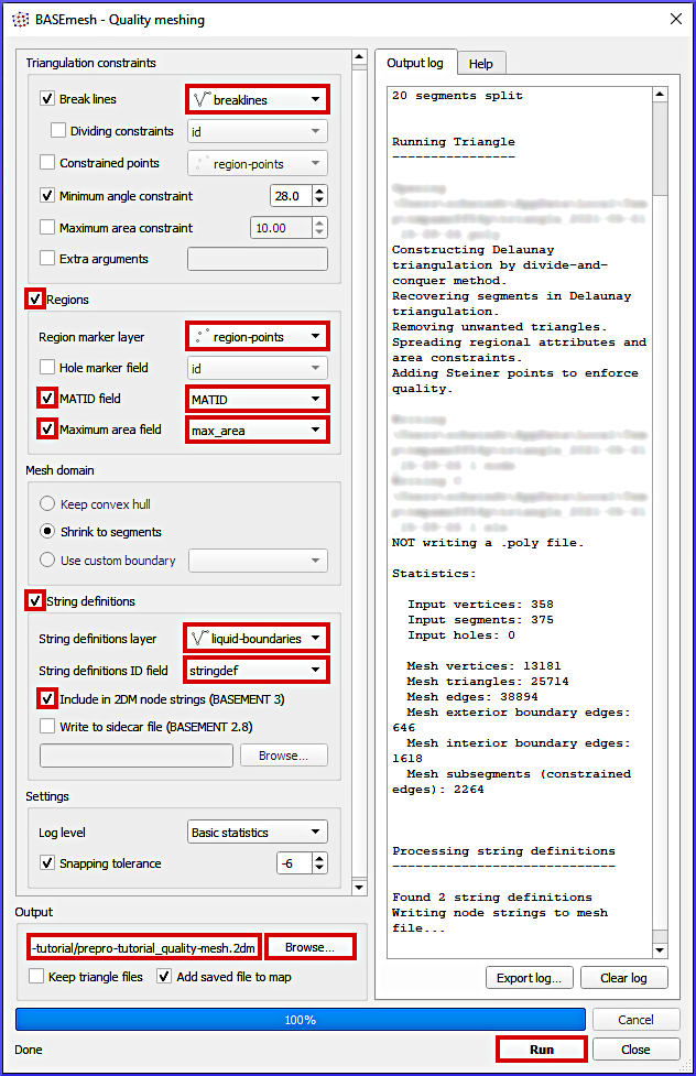
Fig. 106 Definitions to be made in BASEmesh’s Quality meshing tool.

Quality meshing may take a short while. After a successful mesh generation the file prepro-tutorial_quality-mesh-interp.2dm will have been generated and it automatically shows up in QGIS as a single-color surface with 0-0 Bed Elevation. The next section shows the interpolation of elevation data with the BlueKenue^TM software.

Troubles with running the quality mesh generator?

Download the tutorial quality mesh file and save it in the project folder, for instance, /ProjectHome/meshes/prepro-tutorial_quality-mesh-utm33n.2dm.

BlueKenue

Get Started

This section features the BlueKenue software to interpolate terrain elevations from a DEM.xyz file on an SMS 2dm mesh, export the mesh to the SELAFIN/SERAFIN (*.slf) geometry format for TELEMAC, and define boundary lines.

In addition, the Meshing with BlueKenue section explains the mesh generation with BlueKenue^TM, which might be unstable because of program crashes and inflexible for correcting line drawing errors. Still, meshing with BlueKenue^TM might be desirable to create a computational mesh with long triangular cells that approximately follow the river streamlines (i.e., using a channel sub-mesh).

To familiarize with BlueKenue^TM, launch the software (more details in the installation chapter) and locate

• the WorkSpace browser (on the left of the window),

• the Data Items entry in the WorkSpace, where file objects will be listed,

• the Views entry in the WorkSpace, where a 2D View (1) entry appears by default and a 3D View can be added from the Window top menu > New 3D View.

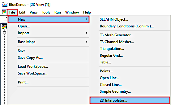
Have a look at the File menu, which enables to:

• Create New BlueKenue^TM objects, such as SELAFIN, Conlim Boundary Condition, T3 Mesh Generator, or 2D Interpolator objects.

• Open file types such as *.slf geometry files or *.xyz point clouds.

• Import files such as:

  • an ArcView Shapefile (read more about shapefiles),

  • an SMS 2dm Mesh like the one created in the above pre-processing with QGISsection, or

  • a GeoTIFF raster, which will not work with many GeoTIFF rasters in practice because BlueKenue^TM cannot handle Float32 or Float64 data in a GeoTIFF.

The Edit menu enables editing BlueKenue^TM objects, such as lines, point sets, or meshes.

The Tools menu provides routines that can be applied to particular BlueKenue^TM objects or for combining objects. In particular, this tutorial will make use of the Map Objects… tool.

Files and Objects

BlueKenue^TM saves every object in software specific file formats and this eBook refers to the following BlueKenue^TM file objects (alphabetic order of file endings):

• *.bc2 files contain Conlim Boundary Conditions.

• *.cli files contain ready-to-use boundary conditions for TELEMAC and can be produced with a *.bc2 object.

• *.i2s files contain closed or open lines.

• *.in2 files contain 2D Interpolators for mapping elevation (or other) data on a mesh.

• *.slf files contain ready-to-use TELEMAC meshes that stem from a BlueKenue^TM SELAFIN object and a *.t3s mesh file.

• *.t3c files contain BlueKenue^TM channel mesh generator objects.

• *.t3m files contain BlueKenue^TM mesh generator objects to create a *.t3s mesh object.

• *.t3s files contain BlueKenue^TM mesh objects that can either be imported (e.g., from an SMS 2dm file) or created with a *.t3m mesh generator.

All files that are created with BlueKenue^TM are based on the ASCII EnSim 1.0 file type standard. The EnSim Core builds on HDF and it is documented in BlueKenue^TM’s user manual PDF that comes along with the BlueKenue installer (in BlueKenue^TM press the F1 key to open the manual). Note that understanding the EnSim Core can significantly facilitate troubleshooting structural errors of BlueKenue^TM files.

Load XYZ Points

Download the provided dem.xyz point cloud that contains EnSim-formatted 3d coordinates of the river ecosystem DEM that will be modelled in this tutorial. The *.xyz file was derived from the GeoTIFF DEM used in the QGIS pre-processing.

The .xyz file is not an XYZ tile

The point cloud in the *.xyz file is different than the regular XYZ tile raster that constitutes the satellite imagery basemap.

To load the dem.xyz file in BlueKenue^TM, open it from the File menu (File > Open…) and take the following actions in the popup window:

• Navigate to the download folder.

• Next to the File name: field, locate the file type drop-down menu and change the default from Telemac Selafin File (*.slf) to Point Sets (*.pt2, *.xyz, *.pcl).

• Click Open to finalize the import.

To verify if the point cloud was correctly imported, drag the new dem (Z) data items to the 2D View (1) entry. Figure 107 shows the imported XYZ point cloud in BlueKenue^TM.

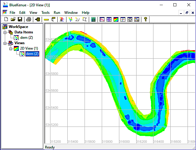
Fig. 107 The provided dem.xyz imported in BlueKenue^TM.

To verify the CRS of the point dataset, right-click on dem (Z), select properties, go to the Spatial tab, and make sure that BlueKenue^TM correctly identified UTM Zone 33 in the Coordinate System frame and WGS 84 as Ellipsoid.

BlueKenue Meshing (Optional)

Skip this section if you created a .2dm quality mesh with BASEMESH

This is an optional section for users who do not want to use QGIS and the BASEmesh plugin for meshing. Generating a mesh with BlueKenue^TM can be useful, for instance, to produce a computational grid that has triangular cells oriented parallel to the riverbanks (i.e., a channel sub-mesh). Otherwise, if the *.2dm mesh file was created with QGIS, jump to the section on creating a Selafin Object.

This section features the basic mesh generation with BlueKenue^TM, which also runs smoothly on Linux through the PlayOnLinux app. Additionall, the Baxter tutorial [GML13] provides more details for getting started with BlueKenue along with detailed screenshots.

Draw Model Boundary (Closed Line)

Delineate the model boundary (outline) with a closed line object (see also Fig. 108):

• Create a new Closed Line by clicking on the symbol in the BlueKenue^TM menu.

• Draw the new closed line:

  • Make points by clicking close to the outer extent of the dem (Z) layer in the 2D Views (1) window. Ensure that no point lies outside the region where elevation data is available (i.e., tightly delineate dem (Z)).

• Finalize the closed line by pressing Esc.

• Name the closed line, for instance, model-outline.

• Skip Adding a New Attribute by just clicking OK.

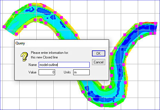
Fig. 108 The Closed Line of the model boundaries in BlueKenue^TM’s 2D View window.

To save the model outline, highlight the new Closed Line object in the WorkSpace browser and click on the disk symbol. Consider creating a new folder called bk-mesh that will contain all BlueKenue^TM objects required for meshing. Thus, save the model outline (Closed Line), for example, as /bk-mesh/model-outline.i2s.

Troubles with drawing the model outline?

The outline can also be downloaded from the supplemental materials repository (download model-outline.i2s). To open the Closed Line from the repository in BlueKenue^TM, go to File > Open… > select Line Sets (*.i2s, *.i3s) as file type and navigate to the download directory.

The current state of BlueKenue^TM can be saved in the form of a workspace.ews file (File > Save WorkSpace… > define a name). Saving the workspace requires that all BlueKenue^TM objects are saved on the disk. Optionally, download the meshing-workspace.ews from the supplemental materials repository.

Loading a WorkSpace

In theory, the saved workspace can be loaded after closing BlueKenue^TM, but the Load WorkSpace… operation often fails for apparently arbitrary reasons. This issue is one of the reasons that make QGIS a better option for meshing.

Draw Open Lines of the Channel Banks

Similar to the above-created breaklines in QGIS, the channel banks can be delineated with Open Line objects. For this purpose create two Open Line objects as follows:

• Create a new Open Line by clicking on the symbol in the BlueKenue^TM menu.

• Draw the new open line:

  • Make points by following the blue-ish-green areas as indicated in Fig. 109 2D Views (1) window (flow direction from left to right).

• Finalize the open line by pressing Esc.

• Name one open line LeftBank and the other RightBank.

• Skip Adding a New Attribute to: by just clicking OK.

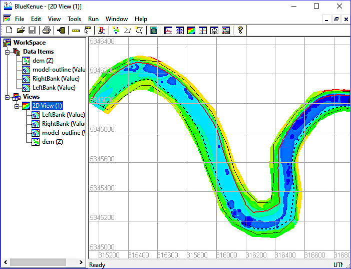
Fig. 109 The finalized Open and Closed Line objects delineating the model boundaries and the channel banks. The RightBank Open Line is represented by the dashed black line and the LeftBank Open Line is represented in red.

Troubles with drawing the open lines of the channel banks?

Download the lines from the supplemental materials repository. Notably download LeftBank.i2s and RightBank.i2s. To open the Open Line objects from the repository in BlueKenue^TM, go to File > Open… > select Line Sets (*.i2s, *.i3s) as file type and navigate to the download directory.

Generate Mesh(es)

BlueKenue^TM provides mesh generators for creating regular or unstructured computational grids (meshes). This example features the T3 Channel Mesher to generate a triangular mesh, which involves first creating a channel mesh (sub-mesh) and second generating a compound mesh that embeds the channel sub-mesh in a coarser mesh of the floodplains. To this end, start with creating a new T3 Channel Mesher object (File > New > T3 Channel Mesher). In the popup window set:

• CrossChannelNodeCount to 20 and

• AlongChannelInterval to 15.

Click OK (not Run) to close the new T3 Channel Mesh window. Next, drag and drop the above-created LeftBank and RightBank Open Line objects on their equivalent attributes of the new T3 Channel Mesh object in the WorkSpace browser as indicated in Fig. 110. Next, generate the channel mesh by double-clicking on the new T3 Channel Mesh object and click Run. To visualize the resulting Mesh, drag it on the 2D View (1) object.

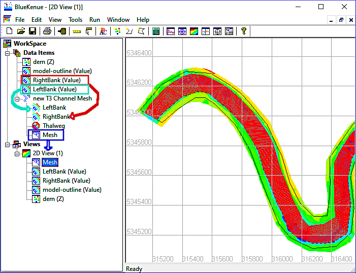
Fig. 110 Create and visualize the channel mesh after dragging the LeftBank and RightBank Open Line Objects on their name equivalents of the T3 Channel Mesh object.

Troubles with creating the channel mesh?

Download the channel-mesh.t3c mesh generator and the channel-mesh.t3s mesh objects from the supplemental materials repository. To open the T3 Mesh object from the repository in BlueKenue^TM, go to File > Open… > select 2D T3 Mesh (*.t...) as file type and navigate to the download directory.

Next, embed the channel mesh in a coarser floodplain mesh by creating a new T3 Mesh Generator object (File > New > T3 Mesh Generator). In the T3 Mesh popup window make the following settings (see also Fig. 111):

• Enable the Resample Outline checkbox.

• Set the Default Edge Length to 20.

• Keep all other defaults.

• Press OK (not Run).

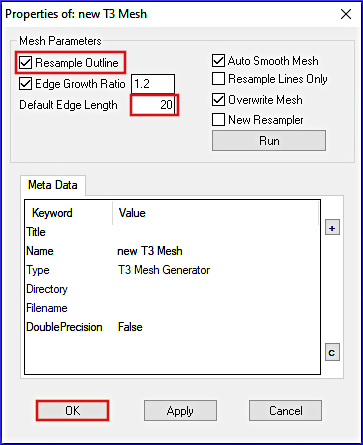
Fig. 111 Setup the properties of the new T3 Mesh Generator object.

Define the Outline (Value) by dragging (see also Fig. 112):

• The above-created model-outline object on the Outline (Value) of the new T3 Mesh, and

• The channel Mesh on the SubMeshes attribute of the new T3 Mesh.

Generate the compound mesh by double-clicking on the new T3 Mesh object and single-clicking on Run. Confirm the question box (Continue? > Yes) and press OK after the mesh generator is finished (Done…). To visualize the resulting Mesh, drag it on the 2D View (1).

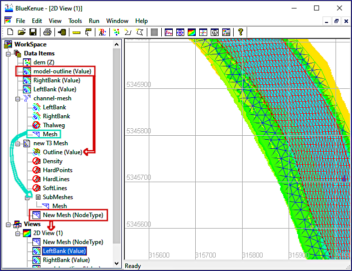
Fig. 112 The compound mesh after dragging the model outline on the Outline (Value) and the channel Mesh on the SubMeshes attribute of the new T3 Mesh generator object.

What is the difference between the channel mesher and the mesh generator?

Figure 112 shows that the channel mesh is streamline-adjusted following the channel banks. This kind of mesh is known to be advantageous for computation speed and model stability. Thus, the availability of the channel mesher in BlueKenue^TM is a strength and the best argument for not using BASEmesh in QGIS for the mesh generation.

Troubles with creating the compound mesh?

Download the compound-mesher.t3m and the compound-mesh.t3s objects from the supplemental materials repository. To open the T3 Mesh object from the repository in BlueKenue^TM, go to File > Open… > select 2D T3 Mesh (*.t...) as file type and navigate to the download directory.

SELAFIN

Open and Import Ingredients

Whether the mesh was created with BlueKenue^TM or QGIS (and the BASEmesh plugin), make sure to have now a BlueKenue^TM workspace with only the XYZ point cloud loaded (see the Load XYZ Points section). Before a SELAFIN object can be created, the previously created mesh (i.e., either the quality-mesh.2dm or the compound-mesh.t3s) needs to be imported into the WorkSpace in addition to the point cloud. The following instructions show the import and use of the *.2dm file:

• In BlueKenue^TM go to File > Import > SMS 2DM Mesh.

• In the import window, navigate to the folder where the *.2dm file lives, select the *.2dm file, and click Open.

• When the Reading SMS 2d Mesh File process is Done…, click OK.

How to load a BlueKenue .T3S mesh file?

In contrast to an SMS 2dm (*.2dm) file that has to be imported, a *.t3s file has to be opened in BlueKenue^TM. To this end, open the T3 Mesh (*.t3s) from File > Open… > select 2D T3 Mesh (*.t...) as file type and navigate to the download directory. Select the *.t3s mesh file and click Open.

Ignore warning messages regarding the projection, but make sure that BlueKenue^TM correctly read the mesh coordinates by dragging the imported (or opened) mesh onto the 2D View (1). The BlueKenue^TM window should now look similar to Fig. 113.

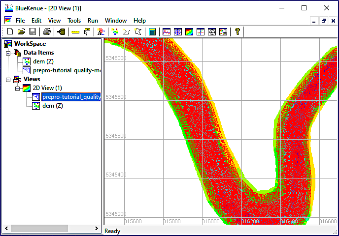
Fig. 113 The imported mesh in the 2D View (1).

Create SELAFIN Object

With the open dem.xyz and the imported (or opened) mesh, all ingredients required by a BlueKenue^TM SELAFIN object are available. Now, create a new SELAFIN object:

• Go to File > New > SELAFIN Object…

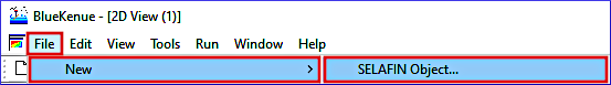
• In the popup window (Properties of:new Selafin) click OK and a new Selafin object will appear in the WorkSpace’s Data Items.

• Right-click on the new Selafin object and select Add Variable…

• Take the following action in the Add New SELAFIN Variable window:

  • In the Mesh field, select the above-imported (or opened) mesh (e.g., prepro-tutorial_quality-mesh-utm33n.2dm).

  • In the Name field, select BOTTOM.

  • In the Units field, select M (i.e., meters).

  • Keep all other defaults and click OK.

• Save the new Selafin object by highlighting it in the Data Item tree of the WorkSpace and clicking the disk symbol. Give the mesh a meaningful and short name, such as qgismesh.slf.

Create 2D Interpolator

A 2D Interpolator object is required to map elevation information onto the Selafin mesh. To this end, create a new 2D Interpolator object and map elevations onto the BOTTOM mesh:

• Go to File > New > 2D Interpolator… and a new 2D Interpolator object will appear in the Data Items of the WorkSpace.

• Drag dem (Z) (i.e., the above-opened dem.xyz pointcloud) onto the new 2D Interpolator object (red arrow in Fig. 114).

• Highlight (click on) the BOTTOM (Anonymous Attribute) mesh attribute of the above-created SELAFIN object (e.g., called qgismesh).

• With the mesh highlighted, go to the Tools top menu > Map Object….

• In the opening Available Objects window select the new 2D Interpolator and click OK.

• Once the Processing… finished, click OK.

• Save the final meshes:

  • The BOTTOM mesh is a BlueKenue^TM *.t3s mesh object; to save it, highlight it in the Data Items tree and click on the disk symbol. Then, save the mesh, for instance, as BOTTOM.t3s file.

  • To save the Selafin mesh in its current (with interpolated elevations) state, highlight the Selafin object (e.g., qgismesh) and click on the disk symbol. This action overwrites the above-saved *.slf file (click Yes to confirm replacing it).

To verify if the 2D interpolator correctly interpolated the elevations on the BOTTOM mesh, drag the BOTTOM mesh onto the 2D View (1). Uncheck the visibility of dem (Z) and the imported (or opened) mesh with a right-click on these elements in the 2D View (1) tree and deselect the Visible entry. Thus, only the height-interpolated mesh should be visible now, as indicated in Fig. 114. If the interpolation has been successful, the mesh is displayed in a variety of (rainbow) colors. Otherwise, if the mesh is completely, monotonously monochrome (red), the elevation interpolation has not been successful and must be repeated (the numerical model cannot work properly without elevation information).

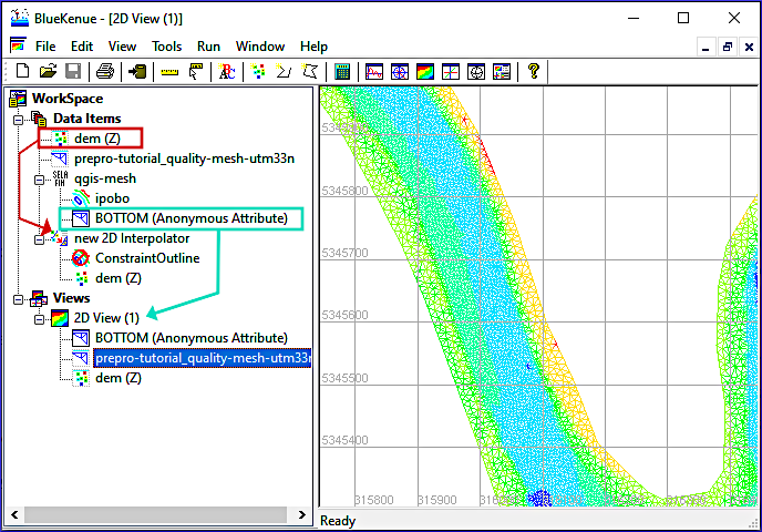
Fig. 114 The height-interpolated mesh in the 2D View (1) with indication of drag and drop actions for running the object mapping with a new 2D Interpolator object.

Troubles with creating the Selafin mesh and or the height interpolation?

Download the BOTTOM mesh and the SELAFIN object from the supplemental materials repository:

• Download BOTTOM.t3s;

• Download qgismesh.slf (EPSG:6173 - ETRS 89 / UTM zone 33N).

Roughness zone interpolation.

Similar to the elevation, friction values can be assigned to created zones with different roughness in the study domain. Read more in the spotlight focus on roughness (friction) zones.

Boundary Conditions (Conlim - CLI)

Create Conlim Object

TELEMAC needs to know how to treat the outer edges of the model (mesh). For this purpose, boundary conditions have to be assigned to all nodes that constitute the *.slfmesh outline:

• Go to File > New > Boundary Conditions (Conlim )… and a new 2D Interpolator object will appear in the Data Items of the WorkSpace.

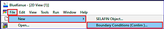
• In the opening popup window (Available t3s Objects), select the above-created BOTTOM mesh (i.e., the mesh with elevation information) and click OK. A new BOTTOM_BC object will occur in the Data Items tree of the WorkSpace.

• Drag the new BOTTOM_BC object onto the 2D View (1), which will enable the prescription of boundary condition types (details in the next section).

Figure 115 illustrates the new BOTTOM_BC object in the 2D View (1) and indicates where upstream and downstream liquid boundaries will be applied in the next section.

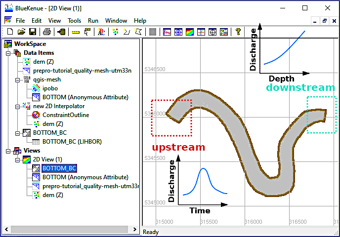
Fig. 115 The new Boundary Conditions (Conlim) object (BOTTOM_BC) in the 2D View (1) with a qualitative overview of the position of upstream and downstream boundaries where prescribed flow (Q) and prescribed flow (Q) and Depth (H) will be applied later in the TELEMAC setup.

To save the new BOTTOM_BC object, highlight it in the Data Items tree and click on the disk symbol. Define a filename such as boundaries.bc2. As a result of saving the object, the BOTTOM_BC object takes on the new file name (e.g., boundaries).

Define Liquid Boundaries

The default boundary type of the boundaries object is Closed boundary (wall). To enable mass (i.e., water, sediment, and/or tracer) fluxes through the model, at least two openings must be drawn into the closed boundary. For this purpose, at least one inflow and one outflow open boundary for liquids must be defined. This tutorial uses this minimum number of required open boundaries (i.e., one upstream inflow and one downstream outflow boundary), which are indicated in Fig. 115.

Liquid boundaries must be defined in BlueKenue

Even though the liquid boundaries are already defined in QGIS (see the QGIS section on Liquid Boundaries), it is always necessary to define the liquid boundaries in BlueKenue^TM to fit the node numbers (IDs) of the Selafin mesh.

The upstream (inflow) liquid boundary will constitute an Open boundary with prescribed Q and H (discharge and water depth corresponding to a stage-discharge relation) with the code 5 5 5 and the downstream outflow (liquid) boundary will constitute an Open boundary with prescribed H with the code 5 4 4 (i.e., prescribed water depth). These types of boundary conditions are required for a dry initialization of the model. In practice, the downstream boundary should be located be at a gauging station where a stage-discharge relation has been calibrated with historic data. To back-calculate cross-section averaged roughness from a stage-discharge relation, take a look at the Python exercise on 1-d hydraulics for solving the Manning-Strickler formula.

Drawing boundary conditions for mass balance

The boundary condition settings affect mass balance, which is a crucial criterion for a sound numerical model. Read more in the spotlight focus on setting up boundary conditions for mass balance. Also, to avoid computational issues, define liquid boundary lines only along the channel bottom as illustrated in the below Fig. 116.

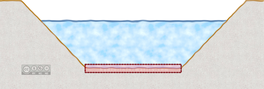
Fig. 116 The red highlighted part of this qualitative cross section should be defined as the inflow (upstream) boundary condition. Mesh nodes at the riverbanks and on the floodplains should not be included.

To assign the two liquid boundary lines, zoom into the downstream and upstream regions indicated in Fig. 115 and create both boundaries as follows (toggle tabs):

Upstream boundary

• Zoom into the upstream region indicated in Fig. 115.

• Locate the main channel banks corresponding to the breaklines drawn in QGIS (see above) or BlueKenue^TM (see above).

• Double-click on a node at one bank of the model outline (no matter what bank), then hold the Shift key and double-click on a node at the other bank to highlight the inflow (purple) line (see Fig. 117).

• Right-click on the purple inflow line and select Add Boundary Segment.

• In the opening window (CONLIM Boundary Segment Editor) make the following settings:

  • Define Boundary Name as upstream.

  • In the Boundary Code field select Open boundary with prescribed Q and H (5 5 5).

  • Keep all other defaults and click OK.

• Save the boundaries object by clicking on the disk symbol and confirm overwriting boundaries.bc2 (i.e., click Yes).

Switch to the Downstream boundary tab to define the outflow conditions according to Fig. 118.

Fig. 117 The upstream boundary definition. Double-click on a node at one bank, then hold the Shift key and double-click on a node at the other bank to highlight the inflow (purple) line. Note that BOTTOM_BC might appear with the name boundaries if the object was saved as boundaries.bc2.

Downstream boundary

• Zoom into the downstream region indicated in Fig. 115.

• Locate the main channel banks corresponding to the breaklines drawn in QGIS (see above) or BlueKenue^TM (see above), which are indicated by the red-dotted lines in Fig. 118.

• Double-click on a node at one bank of the model outline (no matter what bank), then hold the Shift key and double-click on a node at the other bank to highlight the outflow (purple) line (see Fig. 118).

• Right-click on the purple outflow line and select Add Boundary Segment.

• In the opening window (CONLIM Boundary Segment Editor) make the following settings:

  • Define Boundary Name as downstream.

  • In the Boundary Code field select Open boundary with prescribed H (5 4 4).

  • Keep all other defaults and click OK.

• Save the boundaries object by clicking on the disk symbol and confirm overwriting boundaries.bc2 (i.e., click Yes).

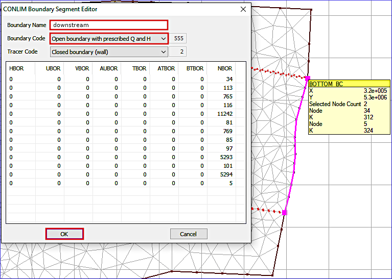
Fig. 118 The downstream boundary definition. Double-click on a node at one bank, then hold the Shift key and double-click on a node at the other bank to highlight the outflow (purple) line. Note that BOTTOM_BC might appear with the name boundaries if the object was saved as boundaries.bc2.

Number of nodes

Make sure that every liquid boundary has at least 5-10 nodes and that every the number of inflow nodes is approximately equal to the number of outflow nodes (in sum), also when defining multiple inflow/outflow boundaries. Read more tips on drawing boundaries in the spotlight focus on boundary conditions.

Ultimately, TELEMAC will need a .cli file (Conlim Table) that can be created by

• highlighting the boundaries (LIHBOR) entry of the boundaries (or BOTTOM_BC) object in the Data Items tree and

• pressing the disk symbol (see Fig. 119).

Save the boundaries file, for instance, as boundaries.cli.

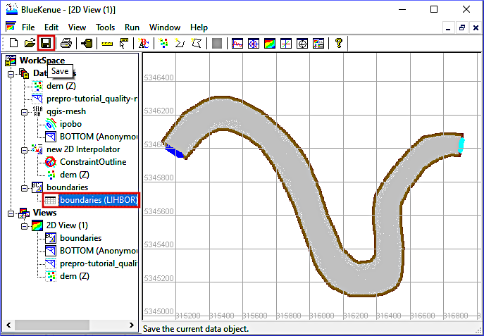
Fig. 119 The finalized boundary conditions are saved in a .cli file by highlighting the boundaries (LIHBOR) entry of the boundaries (or BOTTOM_BC) object in the Data Items tree.

Troubles with creating and defining the liquid boundaries?

Download the boundaries (BOTTOM_BC) BlueKenue^TM and TELEMAC boundaries (LIHBOR)-CLI objects from the supplemental materials repository:

• Download boundaries.bc2;

• Download boundaries.cli.

The here created Selafin/Serafin (*.slf) and boundary conditions (*.cli) files are the main products that are needed for running any other SELAFIN-based TELEMAC tutorial in this eBook. The steady 2d tutorial assigns a constant discharge at the upstream (inflow) and a constant discharge plus constant depth at the downstream (outflow) boundaries. To perform an unsteady calculation, the steady flow rates can be replaced with a *.qsl ASCII text file. To this end, the .cli file can be easily adapted any time later with a basic text editor.