Contributor
This chapter was written and developed by Beatriz Negreiros 
Kernels#
In this section, we will cover fundamental concepts of non-linear classification by introducing the concept of kernels. First, let us recall what we have seen so far in our section about Linear Classification. In linear classification, our task consisted of classifying data points through a hyperplane that could linearly separate the dataset in the features coordinate space. For instance, in a 3d feature space, thus a feature vector such as \((x_1, x_2, x_3) \in \mathbb{R}^3 \), recall that our data is considered linearly separable if there is at least one plane (not line) who can split the points. Unlike linear classification, which assumes a linear relationship between input features and class labels, non-linear classification algorithms use various techniques to capture complex patterns and decision boundaries in the data. In particular, we will look at how we can transform our data into a new coordinate space of higher dimension through kernels, which help us turning the non-linear problem into a linear one.
Kernels allow us to transform data into a higher-dimensional feature space where linear separation becomes possible. One example of ML algorithm that relies on kernels for finding complex pattern and decision boundaries in the data is Support Vector Machine (SVM).
Note
Other non-linear classification algorithms include decision trees, random forests, k-nearest neighbors (KNN), and neural networks. These algorithms employ different techniques different from kernelization to model and capture non-linear relationships between input features and class labels, enabling them to handle complex classification tasks.
Feature transformation#
We will now see how feature transformation works through a 1d example, that is, we have one feature \(x \in \mathbb{R}\). The figure below illustrates the training points (\(n=3\)).
Note from the figure that the dataset is not linearly-separable, at least not in the given feature space in 1 dimension. To turn this problem into a linear-problem, we can perform a feature transformation (\(\phi (x)\)) to look for a decision boundary in a higher-dimensional space. In this particular example, note that we can transform the 1d feature into a new 2d feature vector, where the additional dimension can be seen as a sort of new feature.
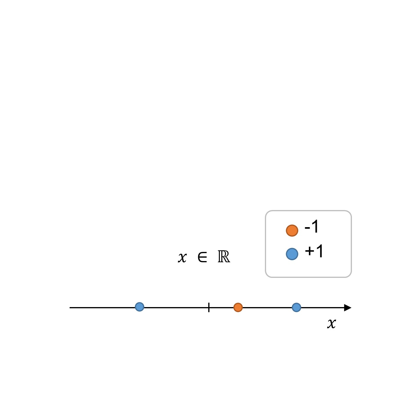
Fig. 253 1: Training datase in the initial feature space.#
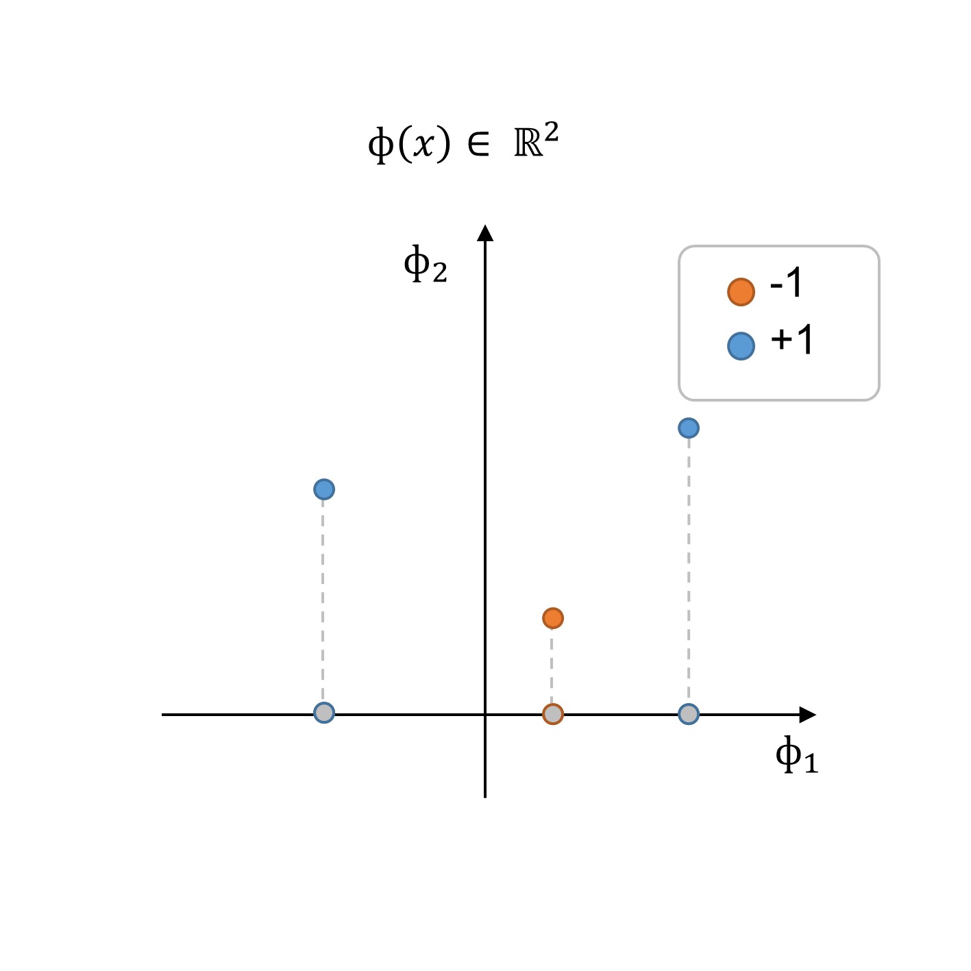
Fig. 254 2: Training dataset in the new feature space \(\Phi(x)\).#
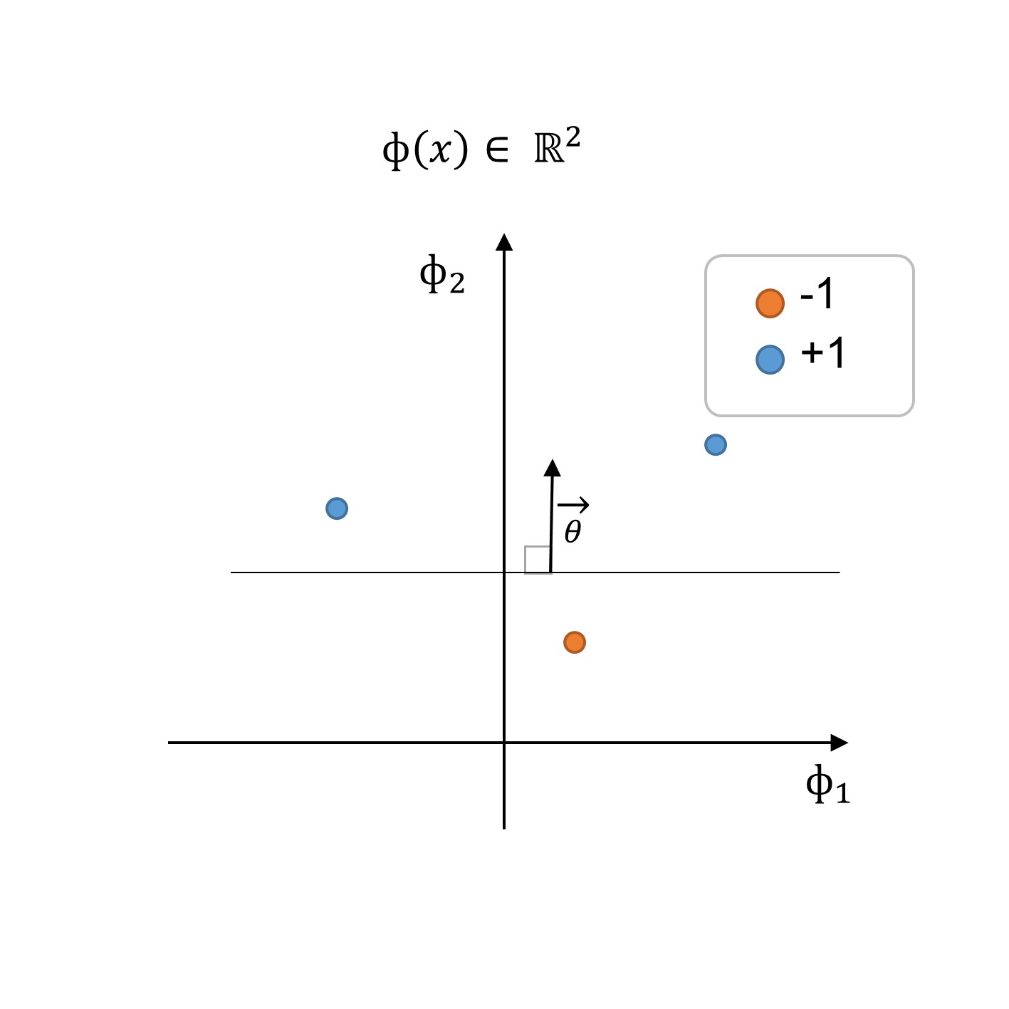
Fig. 255 3: Training dataset and decision boundary in the new feature space \(\Phi(x)\)#
By performing feature transformation as illustrated in the step 2: training dataset in the new feature space \(\Phi(x)\) (see figure above), we can find a classifier \(h(x, \theta, \theta_o)\) with a decision boundary defined by \(\theta\) and the offset parameter \(\theta_0\):
Exercise 1: Feature transformation with kernels
The figure below shows a dataset that is not linearly separable in the original feature space \(x = [x_1, x_2]\). Can you think of a kernel function to create a higher-dimensional feature space where there is a decision boundary solvable through linear classification?
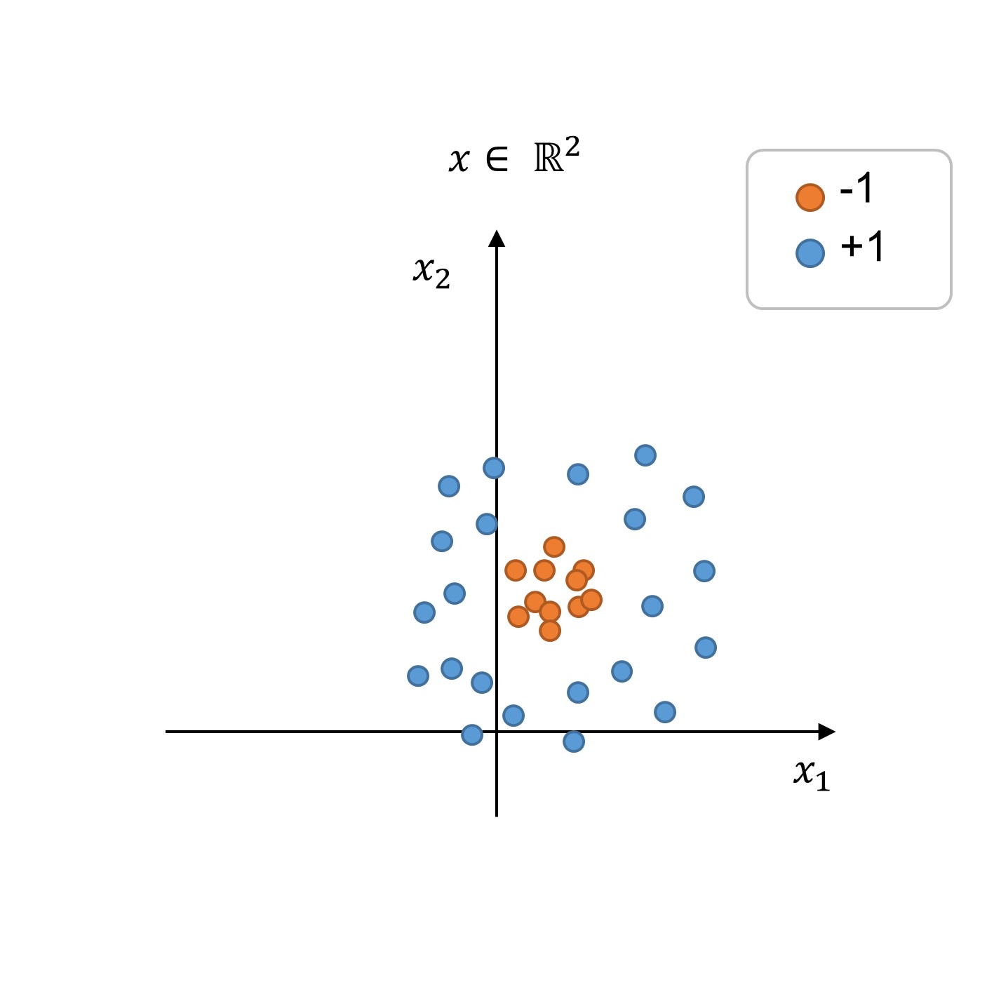
Fig. 256 Exercise 1 on kernels#
Hint
Hint: The points are clearly separable by a circumference in the original feature space \(x \in \mathbb{R}^2\). Now try to draw a kernelized feature space \(\Phi \in \mathbb{R}^3\).
Solution
We start solving this problem by recalling the equation of a circumference not centered in the origin:
Expanding the above equation we obtain:
The terms \(a\), \(b\), and \(c\) are constants, thus we can simplify the equation to:
where \(C = (a^2 + b^2 - c)\).
Note that the above equation denotes our non-linear decision boundary in the original feature space \(x \in \mathbb{R}^2\) and thus should equal the expression \(\theta \cdot \Phi(x) +\theta_0\):
which means that \(\theta_0 = C\), \(\Phi(x) = [x_1 \;\; x_2 \;\; x_1^2 \;\; x_2^2]\), and thus we can also find \(\theta\) in terms of the circumference parameters: