Contributor
This chapter was written and developed by Beatriz Negreiros 
Linear Classification#
In this section, we will cover the fundamentals of linear classification through a simple ML algorithm, the Perceptron. In addition, we will extend the concepts behind the Perceptron algorithm by considering aspects of regularization to build a margin linear classifier.
Requirements
You are familiar with machine learning terms. We recommend reading our introduction to ML section for familiarizing with the nomenclature we use throughout the website.
You are familiar with fundamental linear algebra concepts (such as a dot product, vector projections, planes, eigenvectors and eigenvalues). Please refer to the videos of 3Blue1Brown for a suitable revision if necessary.
Basic knowledge in Python and array computing with NumPy.
Hyperplanes#
Suppose we wish to classify positive and negative objects from the training set of points below (figure on the left):
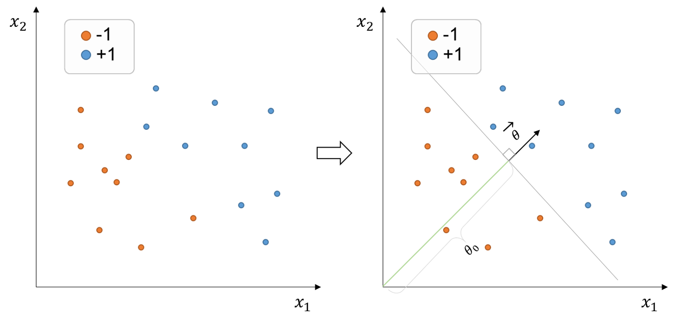
Fig. 248 Training set of points with binary labels (+1, -1) and two-dimensional \((x_1, x_2)\) features. The decision boundary (grey line) is defined by the parameter vector \(\theta\), which is normal to the decision boundary, and offset parameter \(\theta_0\) that linearly separates the data.#
The dataset above is considered linearly separable because it exists at least one linear decision boundary capable of splitting the entire dataset correctly. For instance, we could pass a decision boundary like the grey line above (figure on the right)
In this case, since the features \((x_1, x_2) \in \mathbb{R}^2 \), that is, the feature set belongs to the two-dimensional space, the decision boundary constitutes a line. If we were dealing with a set of features in the three-dimensional space \((x_1, x_2, x_3)\), the decision boundary would be a plane. Analogously, if our feature set were in a higher-dimensional space, the decision boundary would constitute a hyperplane.
A hyperplane with \(d\) dimensions is conventionally denoted by the vector normal to the plane, \(\theta \in \mathbb{R}^d\), and offset (scalar) parameter \(\theta_0\). In the example above, we would define the hyperplane (or decision boundary) as:
Note
Note that \(\theta\) controls the orientation (slope, or inclination) of the boundary, whereas \(\theta_0\) controls the location (or offset, or bias) of the boundary. Thus, if \(\theta_0 = 0\), then the decision boundary crosses the origin. \(\theta_0\) is also often called the bias term.
Our classifier \(h(x, \theta, \theta_0)\) is thus equal to \(sign(\theta \cdot X + \theta_0)\) where \(\theta \in \mathbb{R}^2 \) and \(\theta_0 \in \mathbb{R}\). Recall the sign function, also known as the signum function, is a mathematical function that returns the sign or direction of a real number. That is, if the input number is positive, negative, or 0, the sign function returns +1, -1, or 0, respectively.
Exercise 1
Try to answer whether the pair of training examples below are linearly separable. Which ones are linearly separable through the origin?
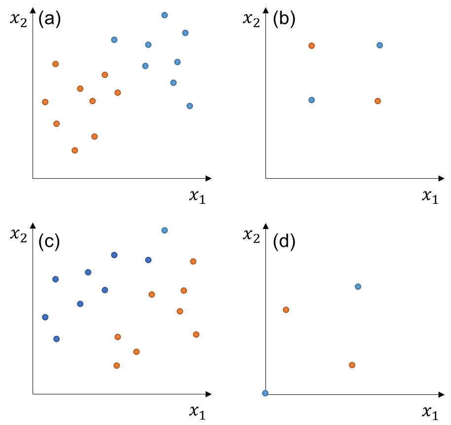
Fig. 249 Exercise 1 on linearly separable pair of examples.#
Solution
Dataset |
a |
b |
c |
d |
|---|---|---|---|---|
Linearly-separable (LS)? |
Yes |
No |
Yes |
No |
LS through origin? |
No |
No |
Yes |
No |
Perceptron algorithm#
In the perceptron algorithm, we typically initialize \(\theta\) as zero (zero vector) and loop through the pair of training examples. At every iteration, we will check if the classifier makes a mistake classifying that training example (i-th example), and if so, then we update the parameters of \(\theta\).
Assume that \(\theta_0 =0\) for simplicity (the decision boundary must pass through the origin). Our perceptron classifier will make a mistake if \(y^{(i)}(\theta \cdot x^{(i)}) \leq 0\). We will then update our \(\theta\) to no longer misclassify that training example. The way to do this is by adding \(y^{(i)}x^{(i)}\) to the previous \(\theta\). Thus, the update would look like:
Exercise 2: Understanding the perceptron update
Try to understand why is this update useful. Hint: substitute the expression for the updates \(\theta\) in the if check.
Solution
Substituting the expression for the updated \(\theta\) to check if the classifier still makes a mistake in that example:
We initialize \(\theta\) as zero, thus the expression is simplified to:
Since any label time itself is equal to one (both \(1 * 1\) and \(-1 * -1\) equal 1), the expression turns into:
This means that that the expression \(y^{(i)}(\theta \cdot x^{(i)}) > 0\) (no mistake). Thus, \(\theta\) was updated so that it doesn’t misclassify the i-th example anymore.
We have in hands a set of different training examples which have the potential to nudge/update our classifier in many directions. Thus, it is possible and even expected that the last training examples cause updates that will overwrite earlier, initial updates. This will result that earlier examples will no longer be correctly classified. For this reason, we need to loop through the whole training set multiple \(T\) times to ensure that all examples are correctly classified. Such iterations can be performed both in order or randomly selected from the training examples.
We can code the algorithm as following:
import numpy as np


# Algorithm always starting to loop from x1
def perceptron(X, y, theta, t_times):
    n_mistakes = 0

    # Initialize list to show the progress (updates) of theta
    progress_theta = []

    # Initialize an array with same size as the total number of examples to count how many mistake are made at each training example
    explicit_mistakes = np.zeros(shape=y.shape[0])

    # Loop through the training set T times
    for t in t_times:

        # Loop through the training examples in order
        for index, x in enumerate(X):

            # Check if the algorithm makes a mistake in the i-th (or index-th) example
            if y[index] * np.dot(theta, x) <= 0:
                # Update theta to no longer misclassify the i-th example
                theta = theta + y[index] * x

                # Save the update theta
                progress_theta.append(theta)

                # Update total number of mistakes
                n_mistakes += 1

                # Update total number of mistakes at the i-th training example
                explicit_mistakes[index] += 1
    print('The perceptron did {} mistakes until convergence'.format(n_mistakes))
    return progress_theta, n_mistakes, explicit_mistakes


if __name__ == '__main__':
    X = np.array([[-1, -1], [1, 0], [-1, 1.5]])
    # X = np.array([[-1, -1], [1, 0], [-1, 10]])

    y = np.array([1, -1, 1])

    t_times = range(0, 100)

    theta = np.array([-1, -1])

    a, b, c = perceptron(X, y, theta, t_times)
Margin boundaries and hinge loss#
As you may have noticed, the perceptron algorithm features no regularization term. The goal was simply to find any decision boundary that can split the data correctly. Here, we will introduce the concept of hinge loss and margin boundaries to transform the problem of learning a decision boundary into an optimization problem considering regularization.
Motivation behind margin boundaries#
Let’s take a look at our previously presented training dataset (figure below). Any decision boundary within the dashed grey lines correctly splits the training examples. However, intuitively, we would like to favor a decision boundary that can maximize the distances between the decision boundary and the training points. The reason to do so is because it’s likely that the points we wish to classify in the future have statistical noise, such that a decision boundary located too close to the training examples is more likely to misclassify slightly changed (noisier) versions of the training examples. In contrast, a classifier that holds a relatively higher margin between the decision boundary and the examples will be probably more successful in classifying future, unseen data.
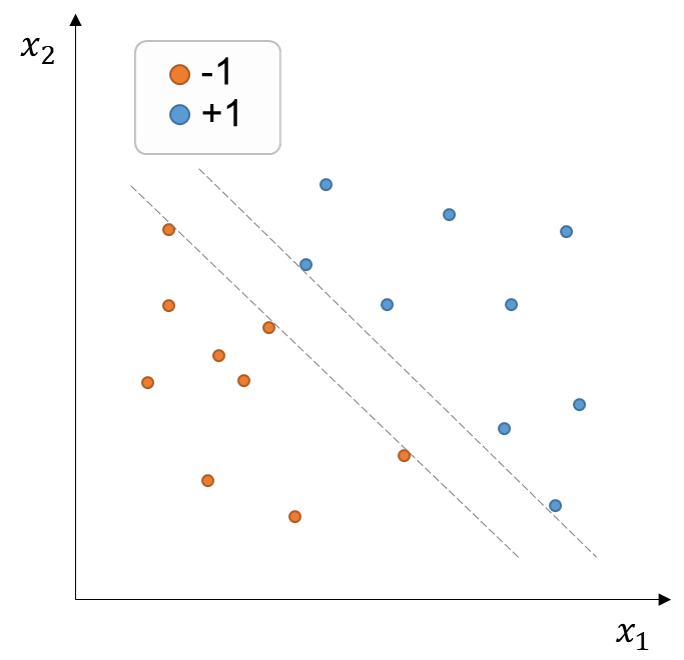
Fig. 250 Training set of points with binary labels (+1, -1) in the two-dimensional feature space \((x_1, x_2)\). Any decision boundary within the dashed grey lines can correctly split the data.#
Optimization problem#
Recall that our goal is to find a linear classifier that maximizes the distances between the decision boundary and the training points (margin linear classifier), but also minimizes the training error. Thus, this constitutes an optimization problem that needs to counterbalance these two factors, which we can state as:
The margins (distances between the decision boundary and the training points) should be maximized.
The training error should be minimized. We will express this in term of hinge loss.
Margin boundaries#
Previously, we saw that the equation defining a decision boundary satisfies \(\theta \cdot X + \theta_0 =0\).
Note
Note that according to \(\theta \cdot X + \theta_0 =0\), any point living exactly at the plane would be misclassified.
We can now define parallel margin boundaries (dashed line in the previous figure) as:
Note that we can define the boundaries like this because we have a degree of freedom in our definition of the decision boundary, namely, the magnitude of the normal vector \(\| \theta \|\). That is, regardless of the value \(\| \theta \|\), our decision boundary remains unaltered.
Recall the problem of computing the smallest distance of a point to a plane. This distance is:
We can now calculate the signed distance between the decision boundary and the i-th example as:
Thus, the distance between the margin boundaries and the decision boundary is:
Hinge loss#
We so far know that \(sign(\theta \cdot x^{(i)} + \theta_0 )\) will classify the i-th example. The way to know if the classification agrees with the label is by multiplying it by \(y^{(i)}\). We can express this agreement also in a slightly modified version, using the hinge loss:
where \(z\) is the agreement (signed distance from the decision boundary) \(y^{(i)}(\theta \cdot x^{(i)}+\theta_0)\).
The figure below illustrates how the hinge loss operates along the z-axis (distance from boundary):

Objective function#
So now we can create an objective function that (1) minimizes the average hinge loss over the training examples, and (2) maximizes \(\frac{1}{\| \theta \|}\). Expression (2) can be also reformulated towards minimizing \(\frac{1}{2}\| \theta \|^2\). Thus we define the objective function as:
where \(\lambda\) is the regularization parameter that balances the importance of minimizing the regularization term \(\frac{\lambda}{2}\| \theta \|^2\) at the cost of incurring more losses (increasing the loss term). Vice versa, the smaller the value of \(\lambda\), the more emphasis we will give to minimizing average loss.
Note
In optimization, the goal is typically to minimize the objective function, and this is also the established convention in ML, although maximizing can also be a valid objective in certain cases.
Exercise 3: Understanding the influence of \(\lambda\)
Try to understand pictorially the influence of the \(\lambda\) parameter on the margin boundaries and decision boundary. Which of the plots showing optimized margin boundaries below are most likely to correspond to a \(\lambda = 1, 10, \mbox{and} \;1000\)
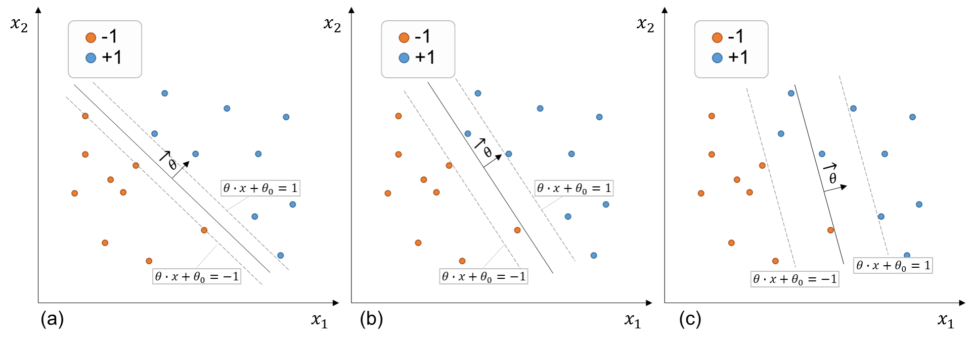
Fig. 251 Effect of the regularization parameter \(\lambda\) on the optimization solution.#
Solution
Plot |
a |
b |
c |
|---|---|---|---|
Lambda value |
1 |
10 |
1000 |