Erste Schritte
Dieser Abschnitt baut auf der SELAFIN (*.slf) Geometrie und den Conlim (*.cli) Randbedingungsdateien auf, die sich aus TELEMAC pre-processing tutorial ergeben. Beide Dateien können auch aus dem ergänzenden Material-Repository dieses eBook heruntergeladen werden:
Download qgismesh.slf (verwendet EPSG:32633 - ETRS 89 / UTM Zone 33N).
Consider saving both files in a new folder, such as /steady2d-tutorial/ that will contain all model files.
Steuerungsdatei (CAS)
The steering file has the file ending *.cas (presumably derived from the French word cas, which means case in English). The *.cas file is the main simulation file with information about references to the two always mandatory files (i.e., the SELAFIN *.slf geometry and the *.cli boundary files) and optional files, as well as definitions of simulation parameters. The steering file can be created or edited with a basic text editor or advanced GUI software such as Fudaa PrePro or BlueKenue. This tutorial uses a basic text editor (e.g., Notepad++ on Windows).
For this tutorial, create a new text file in the same folder where qgismesh.slf and boundaries.cli live, and name it, for instance, steady2d.cas (e.g., /steady2d-tutorial/steady2d.cas). The next sections guide through parameter definitions that stem from the Telemac2d manual. The final steering file can be downloaded from the supplemental materials repository (download steady2d.cas).
Überblick über die CAS-Datei
Das untere Feld zeigt die bereitgestellte steady2d.cas Datei, die für die Ausführung dieses Tutorials verwendet werden kann].
Expand to view the complete .CAS file
/---------------------------------------------------------------------
/ TELEMAC2D
/ STEADY HYDRODYNAMICS TRAINING
/---------------------------------------------------------------------

/ steady2d.cas
/------------------------------------------------------------------/
/			COMPUTATION ENVIRONMENT
/------------------------------------------------------------------/
TITLE : '2d steady'
/
BOUNDARY CONDITIONS FILE : boundaries.cli
GEOMETRY FILE            : qgismesh.slf
RESULTS FILE           : r2dsteady.slf
/
MASS-BALANCE : YES / activates mass balance printouts - does not enforce mass balance
VARIABLES FOR GRAPHIC PRINTOUTS : U,V,B,H,S,Q,F / Q enables boundary flux equilibrium controls, B required for gaia (optional)
/
/------------------------------------------------------------------/
/			GENERAL PARAMETERS
/------------------------------------------------------------------/
TIME STEP : 1.
NUMBER OF TIME STEPS : 15000
GRAPHIC PRINTOUT PERIOD : 200
LISTING PRINTOUT PERIOD : 100
/
/------------------------------------------------------------------/
/			NUMERICAL PARAMETERS
/------------------------------------------------------------------/
/ General solver parameters
DISCRETIZATIONS IN SPACE : 11;11
FREE SURFACE GRADIENT COMPATIBILITY : 0.1  / default 1.
ADVECTION : YES
/
/ STABILITY CONTROLS
PRINTING CUMULATED FLOWRATES : YES
/
/ FINITE ELEMENT SCHEME PARAMETERS
/------------------------------------------------------------------
TREATMENT OF THE LINEAR SYSTEM : 2 / default is 2 - use 1 to avoid smoothened results
SCHEME FOR ADVECTION OF VELOCITIES : 14 / alternatively keep 1
SCHEME FOR ADVECTION OF TRACERS : 5
SCHEME FOR ADVECTION OF K-EPSILON : 14
IMPLICITATION FOR DEPTH : 0.55 / should be between 0.55 and 0.6
IMPLICITATION FOR VELOCITY : 0.55 / should be between 0.55 and 0.6
IMPLICITATION FOR DIFFUSION OF VELOCITY : 1. / v8p4 default
IMPLICITATION COEFFICIENT OF TRACERS : 0.6 / v8p4 default
MASS-LUMPING ON H : 1.
MASS-LUMPING ON VELOCITY : 1.
MASS-LUMPING ON TRACERS : 1.
SUPG OPTION : 0;0;2;2 / classic supg for U and V
/
/ SOLVER
/------------------------------------------------------------------
INFORMATION ABOUT SOLVER : YES
SOLVER : 1
MAXIMUM NUMBER OF ITERATIONS FOR SOLVER : 200 / maximum number of iterations when solving the propagation step
MAXIMUM NUMBER OF ITERATIONS FOR DIFFUSION OF TRACERS : 60 / tracer diffusion
MAXIMUM NUMBER OF ITERATIONS FOR K AND EPSILON : 50 / diffusion and source terms of k-e
/
/ TIDAL FLATS
TIDAL FLATS : YES
CONTINUITY CORRECTION : YES / default is NO
OPTION FOR THE TREATMENT OF TIDAL FLATS : 1
TREATMENT OF NEGATIVE DEPTHS : 2 / value 2 or 3 is required with tidal flats - default is 1
/
/ MATRIX HANDLING
MATRIX STORAGE : 3 / default is 3
/
/ BOUNDARY CONDITIONS
/------------------------------------------------------------------
/
/ Liquid boundaries
PRESCRIBED FLOWRATES  : 35.; 0.
PRESCRIBED ELEVATIONS : 374.80565;371.33
/
/ Type of velocity profile can be 1-constant normal profile (default) 2-UBOR and VBOR in the boundary conditions file (cli) 3-vector in UBOR in the boundary conditions file (cli) 4-vector is proportional to the root (water depth, only for Q) 5-vector is proportional to the root (virtual water depth), the virtual water depth is obtained from a lower point at the boundary condition (only for Q)
VELOCITY PROFILES : 4;1
/
/ Friction at the bed
LAW OF BOTTOM FRICTION : 4 / 4-Manning
FRICTION COEFFICIENT : 0.03 / Roughness coefficient
/ Friction at the boundaries
LAW OF FRICTION ON LATERAL BOUNDARIES : 4 / 4-Manning
ROUGHNESS COEFFICIENT OF BOUNDARIES : 0.03 / Roughness coefficient
/
/ INITIAL CONDITIONS
/ ------------------------------------------------------------------
INITIAL CONDITIONS : 'ZERO DEPTH' / start with dry model conditions
/
/-------------------------------------------------------------------
/			TURBULENCE
/-------------------------------------------------------------------
/
DIFFUSION OF VELOCITY : YES / default is YES
TURBULENCE MODEL : 3
/
&ETAAllgemeine Parameter
Die allgemeinen Parameter definieren die Berechnungsumgebung beginnend mit einem Simulationstitel und den wichtigsten Links zu den beiden obligatorischen Eingabedateien:
BOUNDARY CONDITIONS FILE : boundaries.cli- mit einer MED-Datei, verwenden Sie eine BND-GrenzdateiGEOMETRY FILE : qgismesh.slf
Das Modell output kann mit folgenden Stichworten definiert werden:
RESULTS FILE : r2dsteady.slf- kann entweder eine MED-Datei oder eine SLF-Datei seinVARIABLES FOR GRAPHIC PRINTOUTS(d.h. Ausgabeparameter):U,V,H,S,Q,F, für streamwise (U: ) und lateral (V: ) Geschwindigkeiten, Wassertiefe (H: ), Wasseroberflächenhöhe (S: ), Entladung/Fluxes (Q: ) und Froude-Zahl (F: )Other variables of interest for tutorials in this eBook: bottom elevation
B(required for morphodynamics with Gaia, value of the type of bottom friction usedW(see below), and turbulent kinetic energyK(requires the use of the turbulence model).Die vollständige Liste der verfügbaren Ausgabevariablen finden Sie im Telemac2d Referenzhandbuch, Abschnitt 1.348 (Seite 92).
The velocities (U and V), the water depth (H), and the discharge (Q) are standard variables that should be used in every simulation. In particular, the discharge Q is required to check when (steady) s converge at the inflow and outflow boundaries. Moreover, discharge Q enables to trace integrated fluxes along any user-defined line in the model. The procedure for verifying and identify discharges is described in the discharge verification section in the post-processing.
Die Zeitvariablen (TIME STEP und NUMBER OF TIME STEPS) definieren die Simulationslänge. Die Ausdrucksperioden (GRAPHIC PRINTOUT PERIOD und LISTING PRINTOUT PERIOD) definieren die Ergebnisausgabehäufigkeit. Je kleiner die Ausdruckszeit ist, desto länger dauert die Simulation, da das Schreiben von Ergebnissen ein zeitaufwendiger Prozess ist. Die Ausdrucksperioden (Frequenzen) beziehen sich auf ein Vielfaches des TIME STEPS-Parameters und müssen eine kleinere Zahl als NUMBER OF TIME STEPS sein. Lesen Sie mehr über Zeitschrittparameter im Telemac2d-Handbuch in den Abschnitten 5 und 12.4.2].
In addition, the MASS-BALANCE : YES setting will print out mass fluxes and errors in the computation region, which is an important parameter for verifying the plausibility of the model. Note that this keyword only enables mass balance printouts and does not enforce mass balance of the model, which must be achieved through a consistent model setup following this tutorial and the Telemac2d manual.
Expand to review the GENERAL PARAMETERS used in this tutorial
TITLE : '2d steady flow'
/
BOUNDARY CONDITIONS FILE : boundaries.cli
GEOMETRY FILE : qgismesh.slf
RESULTS FILE : r2dsteady.slf
/
MASS-BALANCE : YES / activates mass balance printouts - does not enforce mass balance
VARIABLES FOR GRAPHIC PRINTOUTS : U,V,H,S,Q,F / Q enables boundary flux equilibrium controls
/
TIME STEP : 1.
NUMBER OF TIME STEPS : 15000
GRAPHIC PRINTOUT PERIOD : 200
LISTING PRINTOUT PERIOD : 100
Allgemeine numerische Parameter
Die folgenden Beschreibungen beziehen sich auf Abschnitt 7.1 im Telemac2d Manual.]
Telemac2d kommt mit drei Solvern zum Approximieren des tiefengemittelten Navier-Stokes-Gleichungen (dh das Flachwassergleichungen) Kundu & Cohen, 2008 (S. 262), das durch Hinzufügen des Schlüsselworts EQUATIONS zur *.cas-Datei ausgewählt werden kann:
EQUATIONS : SAINT-VENANT FEist der Standard, der Telemac2d dazu bringt, eine Finite-Elemente-Methode von Saint-Venant zu verwenden,EQUATIONS : SAINT-VENANT FVmakes Telemac2d use a Saint-Venant finite volume method, andEQUATIONS : BOUSSINESQmakes Telemac2d use the Boussinesq-Approximation, which assumes constant density (incrompressible fluid assumption) and is not to be confused with the Näherung von Boussinesq.
In addition, a type of discretization has to be specified with the DISCRETIZATIONS IN SPACE keyword, which is a list of five integer values. The five list elements define spatial discretization schemes for (1) velocity, (2) depth, (3) tracers, (4) turbulence, and (5) advection (Spalart-Allmaras), respectively. The minimum length of the keyword list is 2 (for velocity and depth) and all other elements are optional. The list elements may take the following values defining spatial discretization:
11(default) aktiviert (lineare) dreieckige Diskretisierung im Raum (d.h. Dreiecke mit drei Knoten),12activates quasi-bubble discretization with 4-nodes, and13aktiviert die quadratische Diskretisierung mit 6-Knoten.
The Telemac2d manual recommend using the default value of DISCRETIZATIONS IN SPACE : 11;11 that assigns a linear discretization for velocity and water depth, which is computationally fast but potentially unstable. The option 12;11 may be used to reduce free surface instabilities or oscillations (e.g., along with steep bathymetry gradients). The option 13;11 increases the accuracy of results, the computing time, memory usage, and it is currently not available in Telemac2d.
In addition, the FREE SURFACE GRADIENT keyword can be defined for increasing the stability of a model. Its default value is 1.0, but it can be reduced close to zero to achieve stability. The developers propose a minimum value of 0., but more realistic results can be yielded by setting this keyword to slightly more than zero (e.g., 0.1). For instance, the following keyword combination may reduce surface instabilities (also referred to as wiggles or oscillations):
DISCRETIZATIONS IN SPACE : 12;11
FREE SURFACE GRADIENT : 0.1
Standardmäßig wird Advektion über das Keyword ADVECTION : YES aktiviert und kann nur für bestimmte Begriffe deaktiviert werden:
ADVECTION OF H : NO / deactivates depth advection
ADVECTION OF U AND V : NO / deactivates velocity advection
ADVECTION OF K AND EPSILON : NO / deactivates turbulent energy and dissipation (k-e model) or Spalart-Allmaras advection
ADVECTION OF TRACERS : NO / deactivates tracer advection
Das Schlüsselwort PROPAGATION (Standard: YES) steuert die Simulation der Ausbreitung und verwandter Phänomene. Zum Beispiel wird das Deaktivieren der Ausbreitung (PROPAGATION : NO) auch Diffusion deaktivieren. Umgekehrt, wenn die Ausbreitung aktiviert ist, kann Diffusion separat deaktiviert werden. Lesen Sie mehr über Diffusion in Telemac2d in der turbulence Sektion.
Finite Elemente
Die folgenden Beschreibungen beziehen sich auf Abschnitt 7.2.1 im Telemac2d Manual.]
Telemac2d verwendet endliche Elemente für iterative Lösungen für Flachwassergleichungen. Das Schlüsselwort BEHANDLUNG DES LINÄREN SYSTEMS ermöglicht es, den ursprünglichen Satz von Gleichungen (Option 1), der am Finite-Elemente-Solver von TELEMAC beteiligt ist, durch eine verallgemeinerte Wellengleichung (Option 2) zu ersetzen. Der Ersatz (d.h. die Verwendung der verallgemeinerten Wellengleichung) ist seit v8p2** auf **Standard eingestellt und verringert die Berechnungszeit, glättet jedoch die Ergebnisse. Dieser Standard (TREATMENT OF THE LINEAR SYSTEM : 2) aktiviert automatisch Massenklumpen für Tiefe und Geschwindigkeit und impliziert eine explizite Geschwindigkeitsdiffusion.
Use SCHEME FOR ADVECTION in lieu of TYPE OF ADVECTION
The TYPE OF ADVECTION keyword is a list of four integers that define the advection schemes for (1) velocities (both and ), (2) water depth , (3) tracers, and (4) turbulence ( or ). The value provided for (2) depth is ignored since v6p0 and a list of two values is sufficient in the absence of (3) tracers and a specific (4) turbulence model. Thus, in lieu of TYPE OF ADVECTION, the SCHEME FOR ADVECTION OF VELOCITIES keyword should be used. The default is TYPE OF ADVECTION : 1;5;1;1 (where the 5 for water depth stems from an older Telemac2d version and does not trigger the PSI scheme). However, the Telemac2d manual indicate that the TYPE OF ADVECTION keyword will be deprecated in future releases.
Die Telemac2d Manual] gibt an, dass die folgenden skalaren SYSTEM FÜR ENTWICKLUNG Schlüsselwörter anstelle der bald veralteten TYP DER ENTWICKLUNG-Liste gelten:
SCHEME FOR ADVECTION OF VELOCITIES : 1 / default
SCHEME FOR ADVECTION OF TRACERS : 1 / default
SCHEME FOR ADVECTION OF K-EPSILON : 1 / default
The three SCHEME FOR ADVECTION scalar keywords may take the following values:
1sets a not mass-conservative method of characteristics (default for all),2setzt ein semi-implizites Schema und aktiviert das Streamline Upwind Petrov Galerkin (SUPG) Schema (mehr unten).3,4,13und14aktivieren das sogenannte NERD-Schema (diese Zahlen aktivieren nur verschiedene Schemata in 3d),5setzt ein massenkonservatives PSI-Verteilungsschema (nicht mit Gezeitenwohnungen verwenden) und15setzt das massenkonservative ERIA-Schema, das mit Gezeitenwohnungen funktioniert.
Optionen 4 und 5 erfordern, dass die Bedingung CFL-Zahl kleiner als 1 ist.
Ohne SYSTEM FÜR DIE GEWINNUNG ... definiert das Schlüsselwort SUPG OPTION (Streamline Upwind Petrov Galerkin) ob Aufwinding zutrifft und welche Art von Aufwinding zutrifft. Die SUPG OPTION ist eine Liste von vier Ganzzahlen, wobei jedes Element einen der folgenden Werte annehmen kann:
0deaktiviert upwinding,1ermöglicht das Aufwinden mit einem klassischen SUPG-Schema (empfohlen, wenn die Bedingung CFL-Zahl unbekannt ist), und2enables upwinding with a modified SUPG scheme, where upwinding equals the CFL-Zahl condition (recommended when the CFL-Zahl condition is small).
Der Standard ist SUPG OPTION : 2;2;2;2, wobei
the first list element refers to flow velocity (default
2),the second to water depth (default
2- set to0whenMATRIX STORAGE : 3),the third to tracers (default
2), andthe last (fourth) to the k-epsilon model (default
2).
Note that the SUPG OPTION keyword is not optional for many keyword combinations and this tutorial uses SUPG OPTION : 0;0;2;2.
Implicitation parameters (IMPLICITATION FOR DEPTH, IMPLICITATION FOR VELOCITIES, and IMPLICITATION FOR DIFFUSION OF VELOCITY) apply to the semi-implicit time discretization used in Telemac2d. To enable cross-version compatibility, implicitation parameters should be defined in the *.cas file. For DEPTH and VELOCITIES use values between 0.55 and 0.60 (default is 0.55 since v8p1); for IMPLICITATION FOR DIFFUSION OF VELOCITY use 1.0 (default).
The default TREATMENT OF THE LINEAR SYSTEM : 2 involves so-called mass lumping, which leads to a smoothening of results. Specific mass lumping keywords and values are required for the flux control option of the TREATMENT OF NEGATIVE DEPTHS keyword and the default value for the treatment of tidal flats. To this end, the mass lumping keywords should be defined as:
MASS-LUMPING ON H : 1.
MASS-LUMPING ON VELOCITY : 1.
MASS-LUMPING ON TRACERS : 1.
In addition, MASS-LUMPING FOR WEAK CHARACTERISTICS : 1. may be defined, which will make Telemac2d using weak characteristics (see below). The default value of any MASS-LUMPING ... keyword is 0. and the maximum value is 1., which makes mass matrices diagonal.
The OPTION OF CHARACTERISTICS keyword defines the method of characteristics that can take a strong (default of 1) or a weak (2) form. A weak form decreases Diffusion, is more conservative, and increases computation time. Telemac2d automatically switches from the default strong (1) to the weak (2) form when
TYPE OF ADVECTIONwird auf1gesetzt,ein beliebiges
SCHEME FOR ADVECTION ...auf1gesetzt ist, oderany
SCHEME OPTION FOR ADVECTION OF ...is set to2.
Keine dieser Optionen sollte mit Tracern verwendet werden, da sie nicht massenkonservativ sind.
Finite Volumen
Die Finite-Volume-Methode wird hier zur Vollständigkeit erwähnt und detaillierte Beschreibungen sind in Abschnitt 7.2.2 des Telemac2d Manual und das Malpasset-Beispiel (telemac/v9.0.0/examples/telemac2d/malpasset/) verfügbar. Um das Finite-Volume-Schema zu aktivieren:
EQUATIONS : 'SAINT-VENANT FV' / the apostrophes are strictly needed hereDie Finite-Volume-Methode beinhaltet die Definition eines Schemas durch das Schlüsselwort FINITE VOLUME SCHEME, das einen der folgenden ganzzahligen Werte annehmen kann:
0ermöglicht das Roe (1981)-Schema,1ist der Standard und ermöglicht das kinetische Schema Audusse et al., 2000,3ermöglicht das Zokagoa & Soulaïmani (2010)-Schema, das mit Gezeitenwohnungen unvereinbar ist,4ermöglicht das Tchamen & Kahawita (1998)-Schema zur Modellierung der Benetzung und Trocknung einer komplexen Bathymetrie,5ermöglicht das Harten Lax Leer-Contact (HLLC) -Schema Toro, 2009 und6ermöglicht das Weighted Average Flux (WAF) Ata, 2012 Schema, für das Parallelität derzeit nicht implementiert ist.
The finite volume/elements schemes are (semi-) explicit and potentially subjected to instability. For this reason, a desired CFL-Zahl condition and a variable timestep are recommended to be defined:
DESIRED COURANT NUMBER : 0.9
VARIABLE TIME-STEP : YES / default is NO
DURATION : 15000
Das Schlüsselwort DURATION ist erforderlich, um die Simulation zu beenden.
The variable timestep will cause irregular listing outputs, while the graphic output frequency is written as a function of the above-defined TIME STEP. Note that this tutorial uses VARIABLE TIME-STEP : NO.
The FINITE VOLUME SCHEME TIME ORDER keyword defines the second-order time scheme, which is by default set to Euler explicit (1). Setting the time scheme order to 2 makes Telemac2d using the Newmark scheme where an integration coefficient may be used to change the integration parameter. Note that NEWMARK TIME INTEGRATION COEFFICIENT : 1 corresponds to Euler explicit. To implement these options in the steering file, use the following settings:
FINITE VOLUME SCHEME TIME ORDER : 2 / default is 1 - Euler explicit
NEWMARK TIME INTEGRATION COEFFICIENT : 0.5 / default is 0.5
Andere Tutorials und das Telemac-Forum empfehlen jedoch die Verwendung der folgenden Schemaeinstellungen für endliche Volumes:
FINITE VOLUME SCHEME : 5 / HLLC
FINITE VOLUME SCHEME SPACE ORDER : 1
FINITE VOLUME SCHEME TIME ORDER : 1
Zusätzliche keyword-empfehlungen für das finite volumenschema sind die folgenden.
OPTION FOR THE DIFFUSION OF VELOCITIES : 2 / only option to get mass conservation but can cause problems with tidal flats
SCHEME FOR ADVECTION OF VELOCITIES : 3 / use 3, also for FV - MATRIX STORAGE must be 3
SCHEME OPTION FOR ADVECTION OF VELOCITIES : 4 / overrides SUPG OPTION and OPTION FOR CHARACTERISTICS
NUMBER OF CORRECTIONS OF DISTRIBUTIVE SCHEMES : 2 / increase for higher accuracy and longer computing time, requires SCHEME OF ADVECTION 3,4,5, or 15 and OPTION 2,3,4
TYPE OF SOURCES : 2 / 2=Dirac is the only possibility for mass conservation, the default=1 means linear function and is not mass conservative
CONTINUITY CORRECTION : YES / particularly important when not only discharge but also depth is imposed at boundaries
Je nach Art der Analyse können auch die lösemittelbezogenen Parameter SOLVER, SOLVER OPTIONS, MAXIMUMNUMMER DER ITERATION FÜR SOLVER und TIDAL FLATS geändert werden. Konkret werden alle ** TIDAL FLAT ** Keywords mit dem FV-Schema ** veraltet.
Numerische Solvenzparameter
Die folgenden Beschreibungen beziehen sich auf Abschnitt 7.3.1 im Telemac2d Manual.]
Der Solver kann mit den Schlüsselwörtern SOLVER, SOLVER FOR DIFFUSION OF TRACERS und SOLVER FOR K-EPSILON MODEL ausgewählt und spezifiziert werden, wobei die folgenden Einstellungen empfohlen werden:
SOLVER : 1 / default is 3
SOLVER FOR DIFFUSION OF TRACERS : 1
SOLVER FOR K-EPSILON MODEL : 1
Das Setzen des SOLVER auf 1 anstelle des Standardwerts von 3 wird mit TREATMENT OF THE LINEAR SYSTEM : 2 (d.h. dem Standard seit v8p2) für konsistente und rückwärtskompatible Steuerungsdateien empfohlen.
Every solver keyword can take an integer value between 1 and 8, where 1-6 use conjugate gradient methods:
1sets the conjugate gradient method for symmetric matrices,2sets the conjugate residual method,3sets the conjugate gradient on normal equation method,4sets the minimum error method,5sets the squared conjugate gradient method,6setzt die Methode des stabilisierten Bikonjugatgradienten (BICGSTAB),7setzt die Generalised Minimum RESidual (GMRES) Methode und8setzt den Yale University Direct Solver (YSMP), der nicht mit Parallelismus kompatibel ist.
Die GMRES-Methode kann mit dem Finite-Elemente-Schema mit den folgenden Lösungsoptionen für Krylowraum aktiviert werden:
SOLVER OPTION : 2 / hydrodynamic propagation
SOLVER OPTION FOR TRACERS DIFFUSION : 2 / tracer diffusion
OPTION FOR THE SOLVER FOR K-EPSILON MODEL : 2 /  k-e or Spalart-Allmaras
Die Lösungsoptionen variieren zwischen den Werten 2 für ein kleines Mesh und 5 für ein großes Mesh. Integer von 3 oder 4 können für mittelgroße Maschen verwendet werden. Das Telemac2d Manual] empfiehlt, Simulationen mehrmals auszuführen, um einen optimalen Wert zu finden, wobei höhere Werte (in der Nähe von 5) die für eine Iteration erforderliche Zeit erhöhen, aber zu einer schnelleren Konvergenz führen.
Numerische Genauigkeit
Die folgenden Beschreibungen beziehen sich auf Abschnitt 7.3.2 im Telemac2d Manual.]
Die Genauigkeitsschlüsselwörter lassen Telemac2d eine Iteration stoppen, wenn zwei aufeinanderfolgende Lösungen für dasselbe Element um weniger als einen ACCURACY-Schwellenwert variieren. Zu diesem Zweck können die folgenden Standardgenauigkeitsschwellenwerte variiert werden (Telemac2d ignoriert nicht relevante Parameter):
SOLVER ACCURACY : 1.E-4 / propagation steps
ACCURACY FOR DIFFUSION OF TRACERS : 1.E-6 / tracer diffusion
ACCURACY OF K : 1.E-9 / diffusion and source terms of turbulent energy transport
ACCURACY OF EPSILON : 1.E-9 / diffusion and source terms of turbulent dissipation transport
ACCURACY OF SPALART-ALLMARAS : 1.E-9 / diffusion and source terms of the Spalart-Allmaras equation
In experience, the solver accuracy should not be larger than 1.E-3 (10). In contrast, very small accuracies will lead to longer computation times. In addition or alternatively to the accuracy keywords, the following default numbers of maximum iterations can be modified to speed up calculations:
MAXIMUM NUMBER OF ITERATIONS FOR SOLVER : 100 / maximum number of iterations when solving the propagation step
MAXIMUM NUMBER OF ITERATIONS FOR DIFFUSION OF TRACERS : 60 / tracer diffusion
MAXIMUM NUMBER OF ITERATIONS FOR K AND EPSILON : 50 / diffusion and source terms of k-e or Spalart-Allmaras
Telemac2d druckt Warnmeldungen aus, wenn die Konvergenz mit der definierten Kombination aus Genauigkeit und maximalen Iterationsnummernschlüsselwörtern nicht erreicht werden konnte. Die ausdrucke der warnmeldung können mit dem schlüsselwort *information about solvent * deaktiviert werden, die deaktivierung von konvergenzwarnungen wird jedoch nicht empfohlen.
Tidalflaggen
Die folgenden Beschreibungen beziehen sich auf Abschnitt 7.5 im Telemac2d Manual.]
Das Schlüsselwort TIDAL FLATS (Standard: YES) gilt nur für das finite elements Schema (EQUATIONS keyword) und kann mit finite volumes ignoriert werden. Der Begriff * Gezeiten* kann leicht verwirrend sein, da Gezeitenebenen über Küstenregionen hinaus auftreten können: Gezeitenflachungen können überall dort auftreten, wo Benetzung und Trocknung von Gitterzellen auftreten können oder an Strömungsübergängen (z. B. wenn schnell fließendes Wasser in eine Rückstauzone eintritt). Benetzen und Trocknen sowie Strömungsübergänge treten in fast allen Umgebungen auf, die komplexer sind als eine quadratisch-ähnliche Strömung, und daher wird die Aktivierung von Gezeitenflächen in Telemac2d-Modellen dringend empfohlen. Obwohl die Aktivierung von Gezeitenflächen zu längeren Berechnungszeiten führt, liefert eine Berechnung mit Gezeitenflächen in den meisten Fällen physikalisch vernünftige Ergebnisse.
Das TIDAL FLATS-Keyword ist mit einigen anderen Telemac2d-Keywords verknüpft, die die Stabilität des Modells und die physische Aussagekraft fördern. Die folgenden keyword-setups können im allgemeinen auf (quasi) stetige, reale flüsse und kanäle angewendet werden (im gegensatz zu laborfluten mit vereinfachten geometrien).
TIDAL FLATS : YES
CONTINUITY CORRECTION : YES / default is NO
OPTION FOR THE TREATMENT OF TIDAL FLATS : 1
TREATMENT OF NEGATIVE DEPTHS : 2 / value 2 or 3 is required with tidal flats
Die OPTION FÜR DIE BEHANDLUNG VON TIDALFLATEN akzeptiert ganzzahlige Werte zwischen 1 und 3, um eine der folgenden Optionen auszuwählen:
1erkennt Gezeitenflachungen und korrigiert den freien Oberflächenverlauf.2removes tidal flat elements by using a masking table that eliminates any contribution of concerned mesh elements. This option may affect the mass conservation of the model.3resembles1, but adds a porosity term to half-dry mesh elements. This affects the amount of water in the model, which equals here the depth integral multiplied by the porosity. A user Fortran file may be used to modify the porosity term in theUSER_CORPORsubroutine.
Das Schlüsselwort BEHANDLUNG NEGATIVER DEPTHS (Standard: 1) definiert einen Ansatz zur Eliminierung negativer Wassertiefenwerte, wobei die folgenden ganzzahligen Zahlen verwendet werden können:
0disables any treatment of negative water depths.1glättet konservativ negative Wassertiefen (Standard).Ein float-nummer-schlüsselwort
THRESHOLD FOR NEGATIVE DEPTHS(standardmäßig:0.) ist nur für diese option verfügbar.Setting the threshold to, for instance,
-0.1makes that negative water depths larger (e.g., -0.05 m) than -0.1 meters remain unchanged.
2imposes a flux limitation that strictly ensures positive water depths.3verhält sich ähnlich wie2, aber für das ERIA Advektion-Schema (setzen SieSCHEME FOR ADVECTION OF TRACERSauf4oder5). Diese Option eignet sich für die Modellierung konservativer Tracer.
Matrix Handling
Die folgenden Beschreibungen beziehen sich auf Abschnitt 7.6 im Telemac2d Manual.]
Telemac2d bietet mehrere Optionen für das Matrixhandling, die für bestimmte Solver-Schemata eingerichtet werden müssen.
Das Schlüsselwort MATRIX STORAGE kann auf:
1for using classic element-by-element matrix storage.3for using edge-based matrix storage (default). This default is required when any SCHEME FOR ADVECTION ... keyword is set to3,4,5,13,14, or15, and when any direct SOLVER is set to8.
The additional MATRIX-VECTOR PRODUCT keyword may be used to switch between multiplication methods for the finite element scheme. However, the default value of 1 (vector multiplication by a non-assembled matrix) should currently not be changed because the only alternative (2 for frontal assembled matrix multiplication) is not implemented for parallelism and quasi-bubble discretization.
Grenzbedingungen
Die folgenden Beschreibungen der Reibungsparameter beziehen sich auf Abschnitt 4.2 im Telemac2d Manual.]
Flüssigkeitsrand-Keywords weisen den räumlich definierten flussaufwärts und flussabwärts gelegenen Flüssigkeitsrandlinien in der Conlim (*.cli) Datei created with BlueKenue hydraulische Eigenschaften zu. Dieser Abschnitt enthält die Zuweisung von stationären Flüssigkeitsgrenzen für eine Entladung von 35 m/s. Dazu wird die stromaufwärtige Randbedingung auf eine stetige Zielzuflussrate gesetzt (Offene Grenze mit vorgegebenem Q) und die stromabwärtige Randbedingung erhält ein Wasserstands-Abfluss Beziehung (Offene Grenze mit vorgegebenem Q und H) zugewiesen (recall Fig. 15). Zum Ausführen dieses Tutorials fügen Sie daher die folgenden Schlüsselwörter zur Steuerungsdatei (*.cas) hinzu:
The keyword
PRESCRIBED FLOWRATES : 35.;0.assigns a flowrate of 35 m/s to the upstream boundary edge, and does not impose a flowrate on the downstream boundary edge. The downstreamQprescription of 0.0 makes Telemac2d ignore this value corresponding for the downstream boundary (prescribed depth only).Das Schlüsselwort
PRESCRIBED ELEVATIONS : 374.80565;371.33weist eine Wasseroberflächenhöhe (oder H in Telemac) in Metern über dem Meeresspiegel (m.s.l.) sowohl an den upstream- als auch an den downstream-Grenzen zu.
The order of prescribed flowrates (Q) and (H) values depends on the order of the definition of the boundaries. Thus, the first list element defines values for the upstream and the second list element for the downstream open boundary.
Liquid boundary conditions may be assigned to any open boundary in the *.cli file.
External files instead of PRESCRIBED-keywords
Anstelle einer Liste von semi-kolon-getrennten Zahlen in der Steuerungsdatei können Flüssigkeitsrandbedingungen auch mit einer Flüssigkeitsrandbedingungsdatei im ASCII-Textformat definiert werden. Zu diesem Zweck müssen die Schlüsselwörter LIQUID BOUNDARIES FILE und / oder STAGE-DISCHARGE CURVES FILE in der Steuerungsdatei definiert werden. Externe Dateien sind für die Simulation von quasi-instationären Strömungen erforderlich (z. B. ein Hochwasser-Hydragraph oder Low-Flow-Sequenzen für Lebensräume) und weitere Details finden Sie in den Abschnitten 4.2.5 und 4.2.6 im Telemac2d-Handbuch oder unsteady section in this eBook].
Ein Geschwindigkeitsprofiltyp kann jeder vorgegebenen offenen Grenze Q (Flowrate) oder U (Geschwindigkeit) in Form einer Liste zugeordnet werden, die die gleiche Elementreihenfolge wie die oben definierten PRESCRIBED ...-Schlüsselwörter hat. Zu diesem Zweck können vor- und nachgelagerte Geschwindigkeitsprofile mit dem Schlüsselwort VELOCITY PROFILES definiert werden, das die folgenden Werte akzeptiert:
1is the default option that defines the flow velocity direction at the boundary nodes normal to their edges. This option assigns a length of 1 to the vector and multiplies it with a numeric factor to yield a target flowrate.2liest U- und V-Geschwindigkeitsprofile aus der Randbedingungen-Datei (*.cli), die mit einer Konstante multipliziert werden, um eine Zieldurchflussrate zu erhalten.3imposes the velocity vector direction normal to the boundary and reads the value (UBOR) from the*.clifile, which is then multiplied by a constant to yield a target flowrate.4imposes the velocity vector direction normal to the boundary and calculates the value’s norm proportional to the square root of the water depth. This option can only be used with a prescribed Q open boundary.5imposes the velocity vector direction normal to the boundary and calculates the value’s norm proportional to the square root of a virtual water depth.
With the upstream boundary being a prescribed Q boundary, this tutorial uses VELOCITY PROFILES : 4;1 in the steering file. Read more about options for defining velocity profiles in section 4.2.8 of the Telemac2d manual.
Ursprüngliche Bedingungen
Die folgenden Beschreibungen beziehen sich auf Abschnitt 4.1 im Telemac2d Manual.]
Die Anfangsbedingungen beschreiben den Zustand des Modells zu Beginn einer Simulation. Telemac2d erkennt die folgenden Arten von Anfangsbedingungen, die in der Steuerungsdatei mit dem Schlüsselwort INITIAL CONDITIONS : 'TYPE' definiert werden können, wobei TYPE eine der folgenden sein kann:
ZERO ELEVATIONinitialisiert die freie Oberflächenhöhe bei 0 (Standard). Die anfänglichen Wassertiefen entsprechen somit der Bodenerhebung.CONSTANT ELEVATIONinitializes the free surface elevation at a value defined with an INITIAL ELEVATION keyword that has a default value of0.. Thus, the initial water depths correspond to the subtraction of the bottom elevation from the water surface elevation . The initial water depth is set to zero at nodes where the bottom elevation is higher than defined by the INITIAL ELEVATION keyword.ZERO DEPTHinitializes the simulation with0(i.e., corresponds to bottom elevation). Thus, the model starts with dry conditions, similar as in the BASEMENT tutorial.CONSTANT DEPTHinitialisiert die Wassertiefen mit einem Wert, der durch ein INITIAL DEPTH-Schlüsselwort definiert wird, das einen Standardwert von0.hat.TPXO SATELLITE ALTIMETRYinitialisiert das Modell anhand von Informationen, die von einer benutzerdefinierten Datenbank bereitgestellt werden (z. B. das OSU TPXO-Modell für ocean tides]. Lesen Sie mehr in Abschnitt 4.2.12 des Telemac2d-Handbuchs zur Modellierung mariner Systeme].
Definieren Sie zunächst die anfängliche Wassertiefe als 0 mit dem folgenden Schlüsselwort, was bedeutet, dass das Modell mit einem trockenen Flussbett initialisiert wird:
INITIAL CONDITIONS : 'ZERO DEPTH'Die Simulationsgeschwindigkeit kann deutlich erhöht werden, wenn das Modell bereits einmal bei der gleichen (Anfangs-)Entladung gelaufen ist. Das Ergebnis einer früheren Simulation kann für die Anfangsbedingung mit den Schlüsselwörtern COMPUTATION CONTINUED : YES (Standard ist NO) und PREVIOUS COMPUTATION FILE : *.slf (geben Sie den Namen einer *.slf-Datei an) verwendet werden. Diese Art der Modellinitialisierung wird auch als hotstart bezeichnet. Lesen Sie mehr über Hotstarts in den Abschnitten unsteady simulation und Gaia. Auch Abschnitt 4.1.3 in der Telemac2d-Handbuch enthält Beschreibungen für die Fortsetzung (Hotstart) Berechnungen.
Friktion (Rugheit)
Die folgenden Beschreibungen der Reibungsparameter beziehen sich auf Abschnitt 6.1 im Telemac2d Manual.]
Das Schlüsselwort LAW OF BOTTOM FRICTION definiert ein Rauheitsmodell für topografische Grenzen, das so eingestellt werden kann:
0for no friction.1für die Haaland (1983)-Gleichung, die eine implizite Form der Colebrook & White (1937)-Gleichung ist, die auf dem Darcy-Weisbach-Reibfaktor aufbaut. Dieses Gesetz beinhaltet ein hohes Maß an Unsicherheit, die aus dem experimentellen Datensatz des ursprünglichen Autors stammt.2for the Chézy (1776) roughness that can be similarly used as3and4.3für Strickler (1923)Rauheit (lesen Sie mehr, zum Beispiel im 1d hydraulics exercise), was die Umkehrung von (4) ist.4für Manning (1891)Rauheit (lesen Sie mehr, zum Beispiel im 1d hydraulics exercise), was die Umkehrung von (3) ist.5für das Nikuradse (1933)-Rauheitsgesetz, das gemäß Rijn (2019) 3 entsprechen sollte.6for the logarithmic law of the wall for turbulent flows. This option assumes that the average flow velocity is a logarithmic function of the distance from the wall beyond the viscous and buffer layers. The thickness of these layers is a function of the wall roughness length Von Karmàn, 1930.7für die Colebrook & White (1937)-Gleichung, die den Darcy-Weisbach-Reibfaktor für turbulente Strömungen in glatten Rohren berechnet.
With respect to the 2d applications in this eBook, the most relevant bottom roughness models are 3 Strickler, 1923, 4 Manning, 1891, and 6 (log law). The Nikuradse (1933) roughness law (5) is recommended for 3d simulations (see the Telemac3d tutorial). Friction is more generally referred to as with the general coefficient , which has a particular relevance for Geschiebe transport (cf. morphodynamic calculations with Gaia).
The FRICTION COEFFICIENT FOR THE BOTTOM keyword sets the value for a characteristic roughness coefficient. For instance, when the friction law keyword is set to 3 Strickler, 1923, the friction corresponds to the Strickler roughness coefficient (in fictive units of m s). For rough channels (e.g., mountain rivers) m s and for smooth concrete-lined channels m s. In fully turbulent flows, the Strickler roughness can be approximated with Meyer-Peter & Müller, 1948 where is the grain diameter of which 90% of the surface grain mixture are finer.
This tutorial features the application of a Manning roughness coefficient of = 0.03, which is the inverse of and implemented with:
LAW OF BOTTOM FRICTION : 4 / 4-Manning
FRICTION COEFFICIENT : 0.03 / Roughness coefficient
Expand to see exemplary values for Manning roughness
Table 1 listet beispielhafte Werte für den Manning-Rauheitskoeffizienten basierend auf Aldridge & Garrett (1973) und Arcement & Schneider (1989) auf.
Table 1:Exemplary values for Manning roughness for straight uniform channels.
Oberflächentyp | Materialdurchmesser (10m) | (ms) |
|---|---|---|
Beton | 0,012-0,018 | |
Fester Boden | 0,025-0,032 | |
Grobsand | 1-2 | 0,026-0,035 |
Kies | 2-64 | 0,028-0,035 |
Pflaster | 64-256 | 0.030-0.050 |
Felsblock | 256 | 0,040-0,070 |
Friction zones (regional friction values)
To create zones with different friction values, have a look at the spotlight focus on roughness zones.
In addition, specific roughness conditions should be defined for the liquid boundaries (see above), which should not be changed in the process of model calibration later. To this end, a measured Wasserstands-Abfluss Beziehung is required to back-calculate cross-section averaged hydraulics. For this purpose, take a look at the Python exercise on 1-d hydraulics for solving the Manning-Strickler formula.
LAW OF FRICTION ON LATERAL BOUNDARIES : 3 / integer (3 is Strickler)
ROUGHNESS COEFFICIENT OF BOUNDARIES : 33.3 / float inverse of n_m=0.03Turbulenzen
Die folgenden Beschreibungen beziehen sich auf Abschnitt 6.2 im Telemac2d Manual.]
Turbulence describes a seemingly random and chaotic state of fluid motion in the form of three-dimensional vortices (eddies). True turbulence is only present in 3d vorticity and when it occurs, it mostly dominates all other flow phenomena through increases in energy dissipation, drag, heat transfer, and mixing Kundu & Cohen, 2008. The phenomenon of turbulence has been a mystery to science for a long time, since turbulent flows (read more about the implementation in RANS) have been observed, but could not be explained by the linear equations systems. Today, turbulence is considered a random phenomenon that can be accounted for in linear equations, for instance, by introducing statistical parameters. For instance, when turbulence applies to the depth-averaged Navier-Stokes-Gleichungen a numerical solution for a quantity (e.g., flow velocity) corresponds to . For this purpose, there are a variety of options for implementing turbulence in numerical models Nezu & Nakagawa, 1993.
The horizontal and vertical dimensions of turbulent eddies can vary greatly, especially in rivers and transitions to backwater zones (tidal flats) where the wide horizontal flow dimension (river width ) is significantly larger than the vertical flow dimension (water depth ): . Telemac2d provides multiple turbulence models that can be applied to the vertical and/or horizontal dimensions and defined with the TURBULENCE MODEL keyword being an integer number for one of the following options:
1to use a constant viscosity coefficient (default) for turbulent viscosity, molecular viscosity, and Diffusion. This closure option should not be used with Wasserstands-Abfluss Beziehung open boundaries (i.e., do not use with prescribed Q and H) Wilson et al., 2002.2to use the Elder formula for the Diffusion coefficient . The Elder turbulence closure also yields small errors for Wasserstands-Abfluss Beziehung open boundaries (i.e., do not use this option with prescribed Q and H) Wilson et al., 2002.3to use the two-equation model solving the Navier-Stokes-Gleichungen. The first equation represents a turbulence closure for the turbulent kinetic energy ; the second equation is a turbulence closure for the turbulent dissipation . Both equations express that the sum of change of (I) and in time, and (II) Advektion transport of and equal the sum of (1) Diffusion transport of and , (2) the production rate of /, and (3) the destruction rate of / Launder & Spalding, 1974. The model is a generalization of the mixing length model (see option5) and assumes that the turbulent viscosity is isotropic (valid for many river applications, but not for circular-rotating flows or groundwater) Bradshaw, 1987. Thus, the model introduces two additional equations and requires a finer mesh than the constant viscosity option1, which leads to a longer computation time. Yet, the model generally yields accurate results and small errors with Wasserstands-Abfluss Beziehung open boundaries Wilson et al., 2002. The following default keywords are associated with the model:VELOCITY DIFFUSIVITY : 1.E-6entsprechend der kinematischen Viskosität von Wasser (10ms).TURBULENCE REGIME FOR SOLID BOUNDARIES : 2für raue Wände von geschlossenen Grenzen, um den Wert anzuwenden, der für die Schlüsselwörter ** RECHT DER BOTTOM FRICTION** und ROUGHNESS COEFFICIENT OF BOUNDARIES gewählt wurde (Rückrufabschnitt Friktion (Rugheit)). Für **glatte geschlossene Begrenzungswände ** setTURBULENCE REGIME FOR SOLID BOUNDARIES : 1.INFORMATION ABOUT K-EPSILON MODEL : YESermöglicht die Ausgabe von Informationen über die Verschlusslösung.
4, um das Smagorinsky (1963) (auch bekannt als general circulation) Modell zu verwenden, das aus der Klimamodellierung stammt. Es stellt eine große Wirbelsimulation dar (LES, im Gegensatz zu RANS). Das Smagorinsky (1963)-Modell berücksichtigt nicht Diffusion.5, um ein Mischlängenmodell gemäß Prandtls Theorie zu verwenden, dass eine flüssige Menge ihre Eigenschaften für eine charakteristische Länge konserviert, bevor sie sich mit dem Massenstrom Bradshaw, 1974 vermischt.6to use the Spalart & Allmaras (1992) one-equation RANS model, which solves a single transport equation for a modified turbulent kinematic viscosity , from which the eddy viscosity is derived through a near-wall damping function. The transport equation for includes convection, Diffusion, a production term proportional to the local strain rate, and a destruction term that depends on the distance to the nearest solid wall. Compared to the model, Spalart-Allmaras is computationally lighter (one equation instead of two) but the wall-distance-based destruction term makes adequate near-wall mesh resolution important. The model was originally developed for high-Reynolds-Zahl aerodynamic (aerospace) flows with mild adverse pressure gradients, and is adapted in TELEMAC-2D as a depth-averaged RANS closure. The following keywords apply; note that keywords containingK-EPSILONin their name also govern the Spalart-Allmaras solver:INFORMATION ABOUT SPALART-ALLMARAS MODEL : YESermöglicht die Konsolenausgabe für den SA-Solver (Standard = JA).TURBULENCE REGIME FOR SOLID BOUNDARIES : 2für raue feste Wände (verwenden Sie1für glatte Wände); gleiche Rolle und Werte wie für das -Modell (siehe Friktion (Rugheit)).VELOCITY DIFFUSIVITY : 1.E-6-- kinematic viscosity of water (10 m/s), same role as in the model.ACCURACY OF SPALART-ALLMARAS : 1.E-9-- Konvergenzschwelle für den Diffusions- und Source-Term-Schritt der -Gleichung (Standard 10-9).SCHEME FOR ADVECTION OF K-EPSILONcontrols advection of ; use the same recommendations as for (e.g.,14with tidal flats,4without).Das fünfte Element von
DISCRETIZATIONS IN SPACEsetzt die räumliche Diskretisierung für (Standard11).SOLVER FOR K-EPSILON MODEL,MAXIMUM NUMBER OF ITERATIONS FOR K AND EPSILONundPRECONDITIONING FOR K-EPSILON MODELregieren auch das SA-Solver-System.
Dieses Tutorial verwendet das Modell (3) wegen seiner Popularität und breiten Anwendbarkeit (nicht zu verwechseln mit Korrektheit).
DIFFUSION OF VELOCITY : YES / enabled by default
TURBULENCE MODEL : 3
Ausführen Telemac2d
Mit der Steuerungsdatei (*.cas) ist die letzte notwendige Zutat für den Betrieb einer stetigen hydrodynamischen 2D-Simulation mit Telemac2d verfügbar. Stellen Sie sicher, dass Sie alle erforderlichen Dateien in einem Simulationsordner ablegen (z. B. ~HOMETEL/mysimulations/steady2d-tutorial/). Die erforderlichen Dateien können auch aus diesem eBook steady2d tutorial repository] heruntergeladen werden und umfassen:
Wenn diese Dateien vorbereitet sind, laden Sie die TELEMAC-Umgebung und führen Sie Telemac2d nach den Erklärungen in den nächsten Abschnitten aus.
Ladeumgebung und Dateien
Gehen Sie zum Konfigurationsordner der Telemac-Installation (z.B. HOMETEL/configs/, wobei HOMETEL so etwas wie /home/telemac/v9.0.0/ sein könnte) und laden Sie die Umgebung (z.B. pysource.gfortranHPC.sh - verwenden Sie dasselbe wie für compiling Telemac).
cd ~/telemac/v9.0.0/configs
source pysource.gfortranHPC.sh
If you are using the Hydro-Informatics (Hyfo) Mint VM
Wenn Sie mit Mint Hyfo VM arbeiten, laden Sie die TELEMAC-Umgebung wie folgt:
cd ~/telemac/v8p2/configs
source pysource.hyfo-dyn.sh
Starten einer Telemac2d-Simulation
Um eine Simulation zu starten, wechseln Sie zum Verzeichnis (cd), in dem die Simulationsdateien leben, und führen Sie die Steuerungsdatei (.cas) mit dem telemac2d.py-Skript aus:
cd ~/telemac/v9.0.0/mysimulations/steady2d-tutorial/
telemac2d.py steady2d.cas -s
The -s flag is not strictly needed but useful for revising simulation characteristics, such as fluxes across the liquid boundaries or the total simulation time. It will write a file named steady2d.cas.[...].sortie and can be used for convergence analysis described in the spotlight chapter on quantitative convergence.
Infolgedessen sollte eine erfolgreiche Berechnung mit den folgenden Zeilen (oder ähnlich) in *Terminal * enden:
[...]
                     *************************************
                     *    END OF MEMORY ORGANIZATION:    *
                     *************************************

 CORRECT END OF RUN

 ELAPSE TIME :
                             03  MINUTES
                             44  SECONDS
... merging separated result files

... handling result files
        moving: r2dsteady.slf
... deleting working dir

My work is done
So produzierte Telemac2d die Datei r2dsteady.slf, die nun in post-processing with QGIS oder ParaView analysiert werden kann.
Nachbearbeitung
The post-processing of the steady 2d scenario uses QGIS and the PostTelemac plugin. Alternatively, Telemac results can also be visualized with ParaView or BlueKenue.
Ergebnisse laden und das Q4TS Plugin
Starten Sie QGIS, create a new QGIS project, setzen Sie das Projekt Koordinatenreferenzsystem auf UTM zone 33N, fügen Sie ein Satellitenbild basemap hinzu und speichern Sie das Projekt (z. B. als tm2d-postpro.qgis) in demselben Ordner, in dem sich die Telemac2d-Simulationsergebnisse-Datei befindet (r2dsteady.slf), ähnlich den Beschreibungen im pre-processing tutorial.
Load the r2dsteady.slf geometry file as mesh layer with drag and drop from the Browser panel to the Layers panel. Make sure to import it with its correct georeference: EPSG:32633 (ETRS 89 / UTM zone 33N).
Um mit diesem Abschnitt fortzufahren, stellen Sie sicher, dass das Q4TS-Plugin installiert ist (siehe Anweisungen unter Software Requirements section). Um Ergebnisse ohne das Q4TS-Plugin zu untersuchen, ist direkt jump to the next section. Q4TS ist hilfreich, um SALOME/ParaVis-ähnliche Analysen (z. B. erweitertes Sondieren, Post-Processing-Pipelines, MED-zentrierte Workflows) durch Konversionsverarbeitung durchzuführen:
In Processing > Toolbox laufen slf2med (Q4TS-Anbieter):
Input .slf:
r2dsteady.slfInput .cli (optional): Ihre Grenzdatei, wenn Sie sie mitnehmen möchten
Output .med: speichern
r2dsteady.med
Then open the *.med file in your preferred MED-capable post-processing workflow (ParaVis/SALOME). This is the one Q4TS feature that meaningfully bridges into “real post-processing” outside QGIS.
Querschnittsanalyse (Extraktwerte entlang von Schnittlinien)
Dies ersetzt die alte Routine “Zeichne eine Linie und inspiziere / exportiere” von PostTelemac, ist aber sauberer, weil es eine reproduzierbare CSV aus einer Linienschicht erzeugt.
Erstellen Sie eine Querschnittslinienschicht:
Create a new line layer (GeoPackage recommended) called, for example,
control_sections.Digitalisieren Sie eine oder mehrere Querschnittslinien über den Kanal (vorgelagerte, nachgelagerte, Kontrollabschnitte usw.).
Export von Querschnittswerten aus der Masche in den CSV
Öffnen Verarbeitung > Toolbox und Ausführen Exportieren Sie Querschnittsdatensätze auf Zeilen aus Mesh
Konfigurieren:
Input Mesh Layer:
r2dsteadyDatensatzgruppen: Wählen Sie aus, was Sie analysieren möchten (Beispiele)
WATER DEPTH(Stabilität / Benetzungsverhalten)Geschwindigkeitskomponenten oder Größe (Hydraulik + Stabilitäts-Hotspots)
jede diagnostische Variable, die Sie an die Ergebnisse geschrieben haben (falls verfügbar)
Datensatzzeit:
Aktuelle Canvas-Zeit für “Snapshot”-Checks verwenden oder
Führen Sie mehrmals für bestimmte Zeitstempel aus, die Ihnen wichtig sind.
Lines für Datenexport:
control_sectionsZeilensegmentierungsauflösung: Setzen Sie dies auf etwas, das für Ihre Mesh-Auflösung sinnvoll ist (nicht überproben).
Output: speichern als
*.csv
Open the exported CSV in Libre Office and plot section profiles (e.g., depth vs. chainage, velocity vs. chainage). Repeat for upstream/downstream sections and compare.
Was Ihnen das sagt (Modellleistungswinkel):
abschnittsweise Sicherheitsüberprüfungen (z. B. Tiefen-/Geschwindigkeitsmuster, bei denen Sie sie erwarten),
Hotspot-Erkennung (unphysische Spitzen in der Nähe von Grenzen, um steile Bathymetriegradienten usw.),
“Ist es noch stabil?” überprüft, indem derselbe Abschnitt in mehreren Zeitschritten verglichen wird.
Knotenanalyse (Zeitreihen an Kontrollpunkten)
Für Konvergenz- / Stabilitätsprüfungen sind Punktzeitreihen in der Regel das schnellste Signal.
Erstellen einer Kontrollpunktschicht:
Create a point layer called
control_points.Fügen Sie Punkte an Orten hinzu, die Ihnen wichtig sind:
nahe Zu-/Abflussgrenzen,
in der Nähe von hydraulischen Steuerungen,
in Zonen, in denen eine Instabilität wahrscheinlich ist (flache Bereiche, starke Steigungen, Benetzungs-/Trocknungsfront).
Zeitreihen aus dem Mesh nach CSV exportieren:
Öffnen Sie Processing > Toolbox und führen Sie Export Zeitreihenwerte aus Punkten eines Mesh-Datasets aus
Konfigurieren:
Input Mesh Layer:
r2dsteadyDatensatzgruppen: Wählen Sie die wichtigsten Variablen aus, die Sie überwachen möchten (Tiefe, Geschwindigkeit und alle von Ihnen ausgegebenen Diagnosefelder)
Punkte für den Datenexport:
control_pointsOutput: speichern als
*.csv
Plot the time series in Libre Office and use it as a quick performance dashboard:
Beruht sich Tiefe/Geschwindigkeit auf einen stabilen Wert (stationärer Zustand)?
Sehen Sie Oszillationen oder Spikes (numerische Probleme, Randbedingungen)?
Machen flache Knoten drehen nass / trocken unrealistisch (Benetzung / Trocknung Tuning Problem)?
These extracted series are directly usable in the wet initialization exercise below.
Export nach GeoTIFF
Um die Modellergebnisse in ein GeoTIFF-Raster zu exportieren, gehen Sie zur Processing Toolbox (in QGIS), erweitern Sie den Mesh-Eintrag und öffnen Sie das Rasterize-Mesh-Dataset-Tool. Führen Sie im Popup-Fenster Rasterize Mesh Dataset (Figure 2) folgende Einstellungen aus:
Input Mesh Layer: Wählen Sie die Telemac Results Mesh Layer (
r2dsteady)Datensatzgruppen: Klicken Sie auf die Schaltfläche ... > Wählen Sie in Verfügbare Datensatzgruppen und wählen Sie die gewünschte Anzahl aus. Dieses Tutorial bietet den Export einer Strömungsgeschwindigkeit. Klicken Sie auf OK, um zum Rasterize Mesh Dataset-Tool zurückzukehren.
Datensatzzeit: Klicken Sie auf das Pfeilsymbol nach oben / unten, um nach unten zu scrollen und den letzten Zeitschritt auszuwählen. In einer instationären (d.h. quasi-stationären) Simulation könnten auch andere Zeitschritte von Interesse sein.
Extent: Klicken Sie auf den Dropdown-Pfeil > Berechnen aus Layer > select r2dsteady
Pixelgröße:
1.0(Standard). Bei gröberen oder feineren Maschen sollte die Pixelgröße variiert werden.Ausgabekoordinatensystem: wählen Sie
EPSG:32633(das ist das Koordinatenreferenzsystem des Meshs)Output-Rasterschicht: Klicken Sie auf ..., um zu einem Zielordner zu navigieren und einen Namen für das Raster einzugeben. Hier:
velocity-tmax.tif.Run die Rasterisierung.
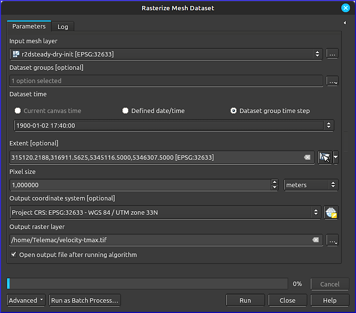
Figure 2:Das Rasterize Mesh Dataset Tool in QGIS
The resulting velocity-tmax raster will be added to the Layers panel. For better visualization, some color is helpful. Therefore, double-click on the new velocity-tmax to open its properties. Go to the Symbology, change the Render type to Singleband pseudocolor, and use your favorite color ramp and number of classes for visualizing the velocity. To make 0-entries invisible, click on their Color symbol and set the Opacity to 0%, or set the Min to 0.0001.
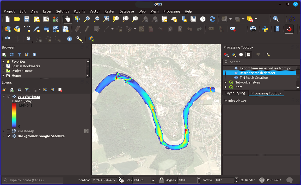
Figure 3:Die exportierte Strömungsgeschwindigkeit (VITESSE) GeoTIFF Raster in QGIS (Hintergrundkarte: Google (n.d.) Satellitenbilder). Der Standort des Raster-Mesh-Dataset-Tools in der Processing Toolbox ist rechts hervorgehoben.
Ergebnisse analysieren
Die erste Analyse der Ergebnisse sollte sich mit der grundlegenden Korrektheit des Modells befassen, beispielsweise in Bezug auf die Massenbilanz und ihre Entwicklung im Laufe der Zeit. Zu diesem Zweck öffnen Sie den Time Controller  im QGIS-Top-Menü.
Quantitative Entlastungskonvergenz
Während der Simulation fließen die Keywords MASS-BALANCE : YES und / oder PRINTING CUMULATED FLOWRATES : YES über Flüssigkeitsgrenzen im Terminal. Um die Flussraten und die Volumenbilanz retrospektiv zu überprüfen, muss die Simulation mit dem Flag -s ausgeführt worden sein, das den Simulationszustand in einer Datei speichert, die ähnlich wie steady2d.cas_YEAR-MM-DD-HHhMMminSSs.sortie aufgerufen wird. Basierend auf der .sortie-Datei können Summen von Flüssen, das Gesamtvolumen und der Volumenfehler mit den Python-Skripten extrahiert und analysiert werden, die zusammen mit der Telemac-Installation bereitgestellt werden (HOMETEL/scripts/python3/). Die Telemac Jupyter Notebooks (HOMETEL/notebooks/ > data manip/extraction/*.ipynb oder workshops/exo fluxes.ipynb) veranschaulichen die Verwendung der Python-Skripte. Eine ausführliche Diskussion über Konvergenz und optimierte Python-Skripte (pythomac]) finden Sie in diesem eBook im Kapitel quantitative Telemac convergence analysis. Mit diesen Skripten wurde Fig. 4 erzeugt, die die Flüsse über die beiden Grenzen der steady-2d-Studie zeigen, was auf eine Konvergenz nach etwa 7000 Zeitschritten hinweist.
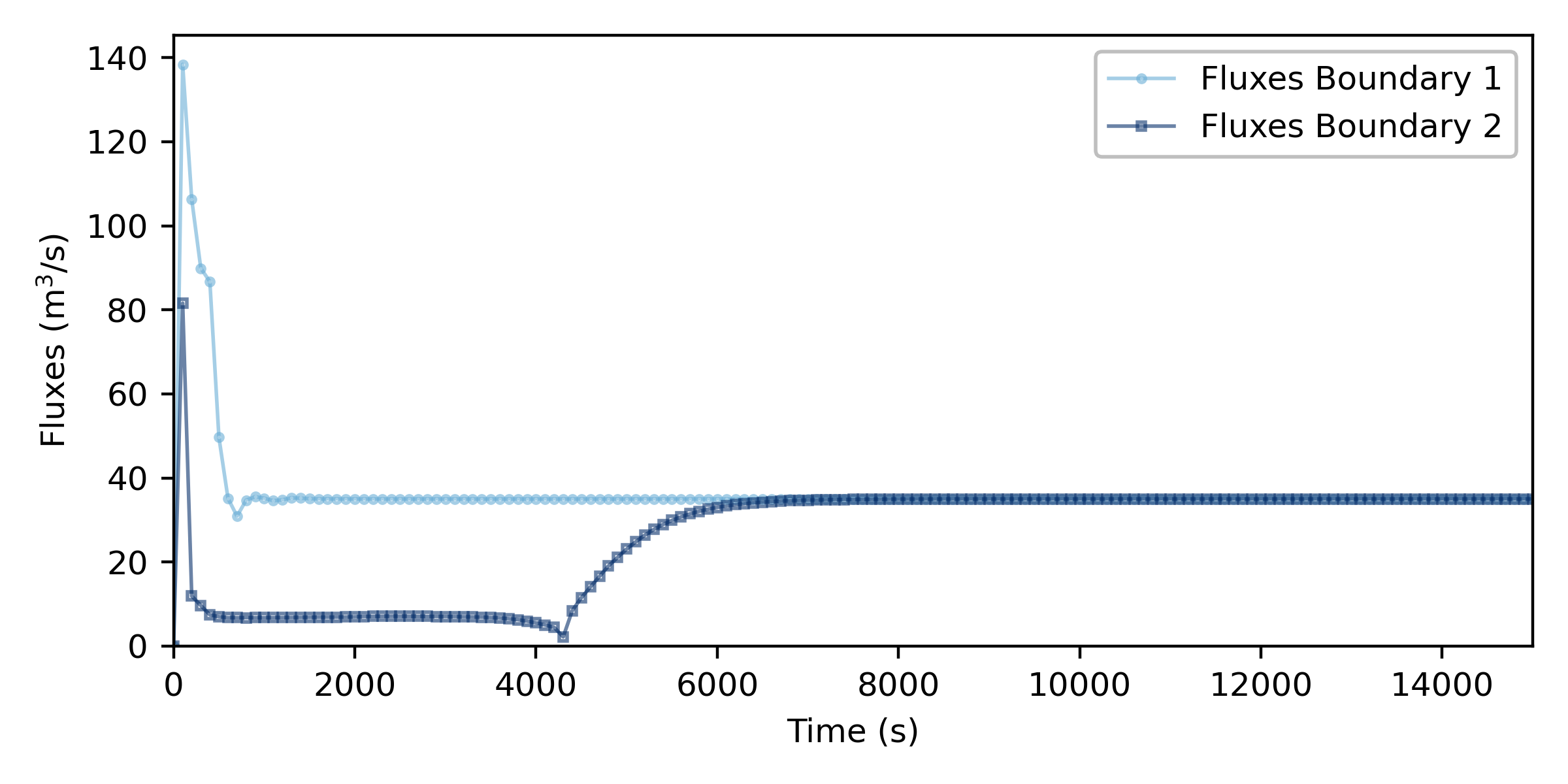
Figure 4:Flusskonvergenzkurve über die beiden Grenzen der trocken initialisierten stationären Telemac2d-Simulation (erstellt mit Pythomac).
Qualitative Geschwindigkeit, Tiefe und Entladung Evolution
The convergence of water depth and flow velocity, and therefore, discharge, can be qualitatively observed in QGIS through the Time Controller (see activation in Fig. 5). The frequency of images can be set through clicking on the cogwheel of the time controller, and image sequences played by clicking in the Play button. Additionally, Fig. 5 uses an overlay of water depth pixel colors (contour plot), and flow velocity vectors, defined in the Layer Styling panel. The North and discharge arrows, and the title are Decorators, which can be found in View > Decorators.
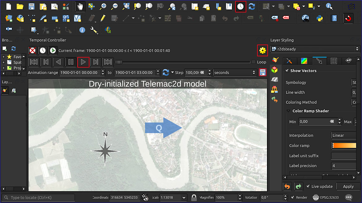
Figure 5:The activated time controller in QGIS enables to move along the time axis of modeled quantities (background map: Google (n.d.) satellite imagery). The red-highlighted buttons activate the time controller, play the sequence of images of selected quantities, provide a setting for playing a frequency of images per second, and enable saving images of all timesteps (see instructions below).
Um eine Reihe von Bildern zu exportieren, um sie in ein filmähnliches GIF zu verwandeln, verwenden Sie die Schaltfläche **Speichern ** des Zeitcontrollers. Richten Sie die gewünschte Auflösung ein und definieren Sie einen Ausgabeordner. Die Serie von PNG-Bildern kann dann beispielsweise mit GIMP] in ein GIF umgewandelt werden. Zu diesem Zweck herunterladen und öffnen GIMP, dann:
Öffnen Sie das erste Bild der exportierten Serie.
Ziehen Sie alle anderen exportierten Bilder in das Layers-Panel von GIMP.
Reverse die Reihenfolge der Layer in GIMP: Layer > Stack > Reverse Layer Order.
Speichern Sie das Bild als GIF: File > Export As....
Select a folder to save the file, in the Name field enter
[any-name].GIF, and click Export.Im Popup-Fenster aktivieren Sie As animation und Loop forever mit einer empfohlenen Verzögerung zwischen Frames von 100 Millisekunden. Behalten Sie alle anderen Standardwerte und klicken Sie auf Export.
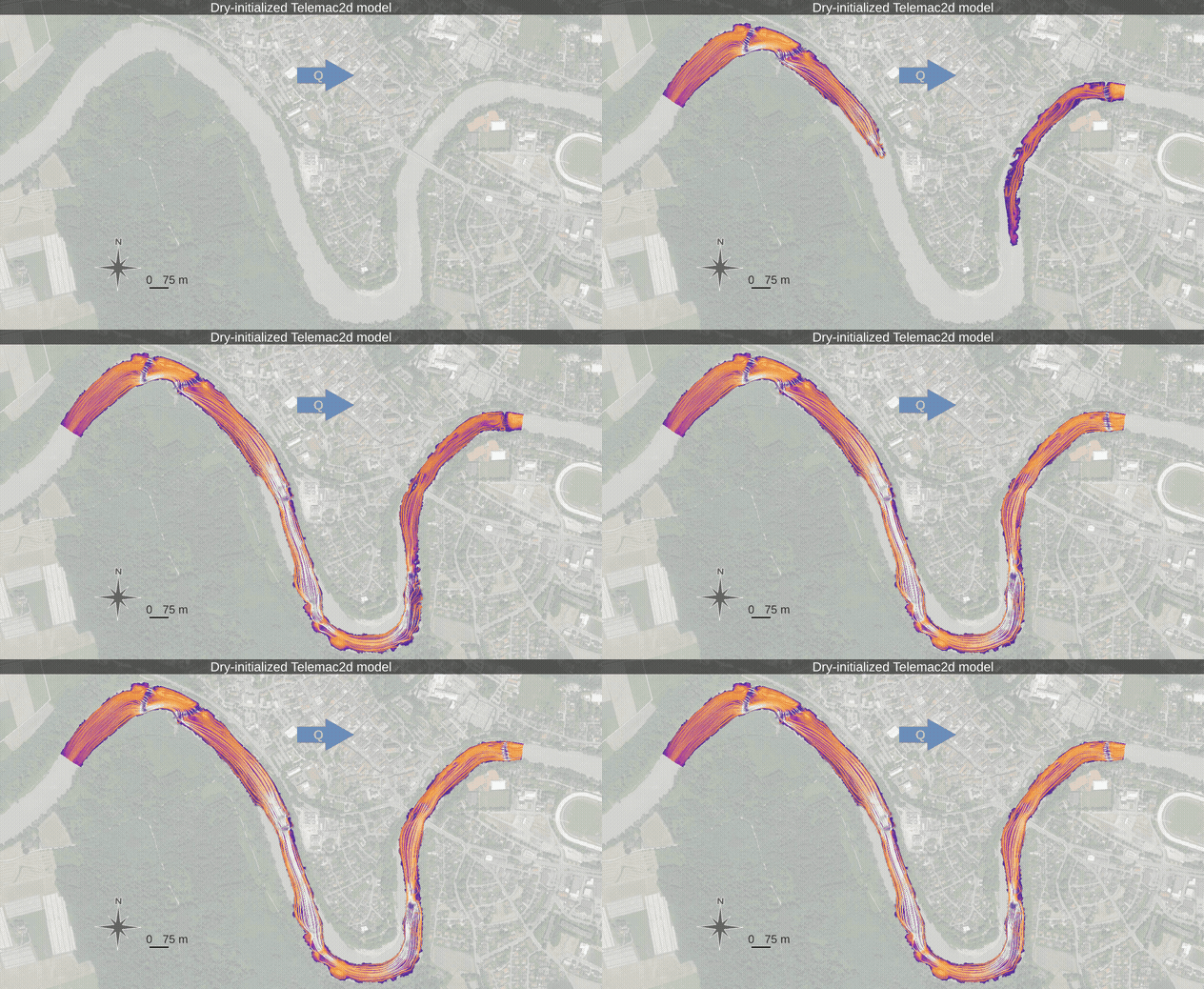
The animated figure below features an exported GIF with water depth in the background and flow velocity as streamline-vectors ranging from 0 to 2.0 m/s. The animation shows how the model is filled from both its upstream (left) and downstream (right) boundaries at the beginning of the simulation. While the upstream discharge was imposed along with a water depth through a 5 5 5 boundary, the downstream boundary only had a prescribed water depth 5 4 4 boundary. The prescription of sufficient water depths was necessary to avoid supercritical flows at the boundaries, which would make the numerical model crash immediately. Because the flux coming from the downstream boundary needs to move uphill, it cannot go very fast and is rolled over by a wave of water coming from the upstream boundary. If a downstream flux was prescribed, the model would have been more unstable and overdetermined.
GIF sequence of a dry-initialized Telemac2d model (large file size!)
Konvertieren in VTK (ParaView)
ParaView is great for 3D analysis. A straightforward way to load TELEMAC .slf result files is to convert them to the .vtk format. One quick way to get this conversion done is by using pputils. To this end, first clone pputils, then make sure the numpy dependency is installed in the same Python environment that you will use for the conversion. Remember where you downloaded pputils:
git clone https://codeberg.org/pprodano/pputils.git
python -m pip install numpy
After that, cd into your TELEMAC model directory (where the .slf file lives) and create a new Python script named slf2vtk.py with the following contents. Make sure to set PPUTILS_DIR to the cloned pputils directory and modify input_slf="results.slf" and output_template="vtk/results.vtk" to your needs:
Click to unroll Python code
"""slf2vtk.py"""
from pathlib import Path
import subprocess
import sys
from typing import List, Optional, Union


PPUTILS_DIR = Path(r"/path/to/pputils").expanduser().resolve()


def slf_to_vtk(
    input_slf: Union[str, Path],
    output_template: Union[str, Path],
    *,
    binary: bool = True,
    start: Optional[int] = None,
    end: Optional[int] = None,
) -> List[Path]:
    """Convert a SELAFIN file to one VTK file per time step."""

    input_slf = Path(input_slf).expanduser().resolve()
    output_template = Path(output_template).expanduser().resolve()

    if not input_slf.is_file():
        raise FileNotFoundError(input_slf)

    if output_template.suffix.lower() != ".vtk":
        raise ValueError("output_template must end in .vtk")

    if "." in output_template.stem:
        raise ValueError("Avoid additional dots in the output filename")

    if (start is None) != (end is None):
        raise ValueError("Specify both start and end, or neither")

    if start is not None and end is not None:
        if start < 0 or end < 0:
            raise ValueError("start and end must be non-negative")
        if start > end:
            raise ValueError("start must be less than or equal to end")

    converter = PPUTILS_DIR / (
        "sel2vtk_bin.py" if binary else "sel2vtk.py"
    )

    if not converter.is_file():
        raise FileNotFoundError(f"PPUTILS converter not found: {converter}")

    output_template.parent.mkdir(parents=True, exist_ok=True)

    command = [
        sys.executable,
        str(converter),
        "-i",
        str(input_slf),
        "-o",
        output_template.name,
    ]

    if start is not None and end is not None:
        # start/end are zero-based time-step indices.
        command += ["-t_start", str(start), "-t_end", str(end)]

    subprocess.run(
        command,
        cwd=output_template.parent,
        check=True,
    )

    pattern = output_template.stem + "[0-9]" * 5 + ".vtk"
    generated_files = sorted(output_template.parent.glob(pattern))

    if not generated_files:
        raise RuntimeError("pputils did not produce any VTK files")

    return generated_files


if __name__ == "__main__":
    generated_files = slf_to_vtk(
        input_slf="results.slf",
        output_template="vtk/results.vtk",
        binary=True,
        # start=0,
        # end=10,
    )

    for path in generated_files:
        print(path)
Führen Sie es dann in einem Terminal aus Ihrem TELEMAC-Modellverzeichnis aus:
python slf2vtk.pyThe value given as output_template is a filename template rather than the name of one final file. For instance, vtk/results.vtk produces vtk/results00000.vtk, vtk/results00001.vtk, and so on; one file for each time step in the .slf file.
By default, the script uses sel2vtk_bin.py to write binary VTK files. Set binary=False to write ASCII VTK files instead. To convert only part of the result series, uncomment start and end; these values are zero-based, inclusive time-step indices rather than simulation times.
Lade TELEMAC-3D Geschwindigkeiten in ParaView
Die im vorhergehenden Workflow erzeugten VTK-Dateien enthalten die Geschwindigkeitskomponenten (u), (v) und (w). Diese Größen repräsentieren die signierten Geschwindigkeiten in der Richtung (x)-, (y)- und (z)-Richtung. Die entsprechende dreidimensionale Geschwindigkeitsgröße ist
Installieren Sie auf einem Debian-Computer ParaView aus dem Debian-Repository, wenn es nicht bereits verfügbar ist, und öffnen Sie dann die konvertierte Dateiserie aus dem Modellverzeichnis:
sudo apt update
sudo apt install paraview

cd /path/to/telemac/model/vtk
paraview --data="$PWD/results..vtk"
In the final command, the two consecutive periods replace the numbered part of files such as results00000.vtk, results00001.vtk, and results00002.vtk. ParaView normally recognizes this naming pattern as a temporal file series. After the reader appears in the Pipeline Browser, select it and click Apply.
Wenn sel2vtk_bin.py oder sel2vtk.py die TELEMAC-Variablen VELOCITY U, VELOCITY V und VELOCITY W erkennt, kombiniert pputils sie in den Punktdatenvektor Velocity.] Um die Gesamtgeschwindigkeit direkt anzuzeigen, wählen Sie Velocity aus dem Menü Coloring und dann Magnitude. Die Vektorkomponenten X, Y und Z entsprechen (u), (v) bzw. (w). Die ursprünglichen Skalar-Arrays bleiben auch als VELOCITY_U, VELOCITY_V und VELOCITY_W verfügbar.
Wenn die Geschwindigkeitsgröße als separates Array zum Clippen, Schwellwerten, Sondieren oder Exportieren benötigt wird, wählen Sie den VTK-Leser im **Pipeline-Browser ** und dann **Filter > Allgemein > Rechner **. Setzen Sie Result Array Name auf VELOCITY_MAGNITUDE, bestätigen Sie, dass die Datenverbindung Point Data ist, und geben Sie Folgendes ein:
mag(Velocity)Click Apply, then color the Calculator output by VELOCITY_MAGNITUDE. For an animation, use Rescale to Data Range over All Timesteps so that one color scale is applied consistently throughout the simulation. This operation reads every time step and may therefore require additional time for a large TELEMAC-3D result set.
Die Syntax der Dateiserie, die Vektorfärbung und der Rechnerausdruck folgen der ParaView data-loading, color-mapping und] Calculator-Dokumentation]. ParaView ist als offizielles Debian package] verfügbar.
Übung: anfängliche Bedingungen
The above Fig. 1 and depth-velocity animation point to stability achieved after approximately 7000 timesteps. A wet-initialized model converges much faster, but either requires a previous run of a dry model initialization, or it can make use of other initial condition keywords in Telemac. Ideally, the dry-initialized model is used as a so-called hotstart condition for a wet-initialized model, as described in the unsteady 2d tutorial.
Anmerkungen zur Kalibrierung
Refresher: Wie funktioniert die Kalibrierung?
Calibration involves the step-wise adaptation of model input parameters to yield a possibly best (statistic) fit of modeled and measured data. In the process of model calibration, only one parameter should be modified at a time by 10 to 20-% deviations from its default value. For instance, if the beginning FRICTION COEFFICIENT : 0.03, the calibration may test for FRICTION COEFFICIENT : 0.033, then FRICTION COEFFICIENT : 0.036, FRICTION COEFFICIENT : 0.027 and so on, ultimately to find out which value for FRICTION COEFFICIENT brings the model results closest to observations.
Darüber hinaus vergleicht eine Sensitivitätsanalyse schrittweise Modifikationen mehrerer Parameter (immer noch: einer nach dem anderen) und deren Auswirkungen auf die Modellergebnisse. Wenn beispielsweise eine 10-%-Variation des FRICTION-COEFFIZIENTEN eine 5-%-Änderung der globalen Wassertiefe ergibt, während eine 10-%-Variation der Gittergröße (Kantenlänge) eine 20-%-Änderung der globalen Wassertiefe ergibt, kann der Schluss gezogen werden, dass die Modellsensitivität in Bezug auf die Gittergröße höher ist. Solche Schlussfolgerungen erfordern jedoch sorgfältige Überlegungen in multiparametrischen, komplexen Modellen von Flussökosystemen.
Kalibrierparameter in Telemac
Die folgenden Parameter können für die Kalibrierung eines 2D-Modells auf Messungen verwendet werden (z. B. Wasseroberflächenhöhe, Wassertiefe oder Strömungsgeschwindigkeitsdaten):
FRICTIONSKOEFFIZIENTER (friction section)
Lösungsmittel, Lösungsoptionen, Implizitation und andere numerische Parameter (numerical parameter section)
Typ des Modells initialization
Nächste Schritte
Make sure the simulation is conservative according to the descriptions in the spotlight chapter on mass balance.
Find a meaningful simulation duration for convergence of a dry-initialized simulation following the algorithms provided with the chapter on quantitative convergence.
Use the dry-initialized model to simulate at least 2-3 steady discharges (with hotstart conditions) for which measurement data is available for calibration and validation.
Das kalibrierte und validierte Modell kann
used for unsteady hydrodynamic simulations, and
dienen als Grundlage für morphodynamic sediment transport modeling with Gaia.
- Kundu, P. K., & Cohen, I. M. (2008). Fluid Mechanics (4th ed.). Elsevier Inc.
- Roe, P. L. (1981). Approximate Riemann solvers, parameter vectors, and difference schemes. Journal of Computational Physics, 43(2), 357–372. 10.1016/0021-9991(81)90128-5
- Audusse, E., Bristeau, M., & Perthame, B. (2000). Kinetic Schemes for Saint-Venant Equations with Source Terms on Unstructured Grids (Research Report RR-3989). INRIA. https://hal.inria.fr/inria-00072657
- Zokagoa, J.-M., & Soulaïmani, A. (2010). Modeling of wetting–drying transitions in free surface flows over complex topographies. Computer Methods in Applied Mechanics and Engineering, 199(33), 2281–2304. 10.1016/j.cma.2010.03.023
- Tchamen, G. W., & Kahawita, R. A. (1998). Modelling wetting and drying effects over complex topography. Hydrological Processes, 12(8), 1151–1182. https://doi.org/10.1002/(SICI)1099-1085(19980630)12:8<;1151::AID-HYP676>3.0.CO;2-Y
- Toro, E. F. (2009). The HLL and HLLC Riemann Solvers. In E. F. Toro (Ed.), Riemann Solvers and Numerical Methods for Fluid Dynamics: A Practical Introduction (pp. 315–344). Springer. 10.1007/b79761_10
- Ata, R. (2012). TELEMAC-2D new finite volume schemes for shallow water equations with source terms on 2D unstructured grids. Proceedings of the XIXth TELEMAC-MASCARET User Conference 2012, 18 to 19 October 2012, St Hugh’s College, Oxford, 93–98. http://henry.baw.de/handle/20.500.11970/104290
- Haaland, S. E. (1983). Simple and Explicit Formulas for the Friction Factor in Turbulent Pipe Flow. Journal of Fluids Engineering, 105(1), 89–90. 10.1115/1.3240948
- Colebrook, C. F., & White, C. M. (1937). Experiments with fluid friction in roughened pipes. Proceedings of the Royal Society of London. Series A - Mathematical and Physical Sciences, 161(906), 367–381. 10.1098/rspa.1937.0150
- Chézy, A. de. (1776). Formula to find the uniform velocity that the water will have in a ditch or in a canal of which the slope is known. In Collection of Manuscripts in the Library of the Ecole des Ponts et Chaussées: Vol. 61 (No. 847) (pp. 165–269). École des Ponts et Chaussées.
- Strickler, A. (1923). Beiträge zur Frage der Geschwindigkeitsformel und der Rauhigkeitszahlen für Ströme, Kanäle und geschlossene Leitungen [Contributions to the question of the velocity formula and the roughness figures for streams, channels and closed pipes]. Mitteilungen Des Eidgenössischen Amtes Für Wasserwirtschaft, Switzerland, 16, 357.
- Manning, R. (1891). Transactions of the Institution of Civil Engineers of Ireland (Vol. 20, pp. 161–207). Civil Engineers of Ireland.
- Nikuradse, J. (1933). Strömungsgesetze in rauhen Rohren [Laws of flow in rough pipes]. VDI Forschungsheft, Beilage Zu “Forschung Auf Dem Gebiete Des Ingenieurwesens,” Ausgabe B, Band 4(361), 26.
- van Rijn, L. C. (2019). Critical movement of large rocks in currents and waves. International Journal of Sediment Research, 34(4), 387–398. 10.1016/j.ijsrc.2018.12.005
- Von Karmàn, T. (1930). Mechanische Ähnlichkeit und Turbulenz [Mechanical similarity and turbulence]. In Third International Congress for Applied Mechanics (Vol. 1, pp. 79–93). Stockholm.