Grundsätze
The calculation of Geschiebe transport requires expert knowledge about the modeled ecosystem for judging whether the system is sediment supply-limited or transport capacity-limited Church & Ferguson, 2015.
Sedimentversorgung begrenzte Flüsse Ein sedimentversorgungsbegrenzter Fluss zeichnet sich durch deutlich sichtbare Schnitttrends aus, die darauf hindeuten, dass der Fluss möglicherweise mehr Sediment transportieren könnte, als im Fluss verfügbar ist. Sedimentversorgung begrenzte Flussabschnitte treten typischerweise stromabwärts von Dämmen auf, die eine unüberwindbare Barriere für Sedimente darstellen. In einem angebotsbegrenzten Fluss ist somit die Flow-Kompetenz (hydrodynamische Kraft oder Transportkapazität) nicht ausreichend, um ein typischerweise grobes Flussbett zu mobilisieren, reicht aber für den Transport externer Sedimentversorgung aus.
- Transport capacity-limited (alluvial) rivers
- A transport capacity-limited river is characterized by sediment abundance where the flow is too small to transport all available sediment during a flood. Sediment accumulations (i.e., the alluvium) are present and the channel tends to braid into anabranches (or to anastomose in fine/sand-dominated environments). Thus, the flow competence (or transport capacity) is insufficient to transport the entire amount of available sediment (external supply and riverbed).
Die folgenden Abbildungen zeigen sedimentangebotsbegrenzte Flussreichweiten und eine transportkapazitätsbegrenzte Flussreichweite.
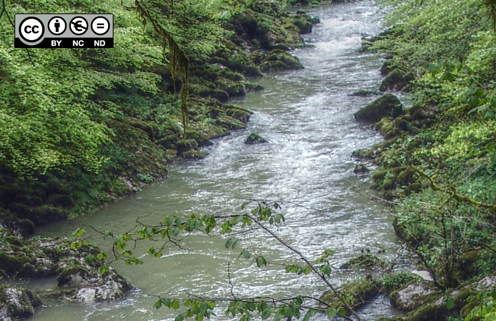
Figure 1:Die Doubs in der Franche-Comté (Frankreich) während einer kleinen Flut. Die Sedimentversorgung wird durch eine Dämmkaskade stromaufwärts unterbrochen mit der Folge eines geraden monotonen Kanals mit signifikantem Pflanzenwachstum entlang der Ufer. Das Flussbett besteht hauptsächlich aus Felsbrocken, die die meiste Zeit unbeweglich sind. Somit kann der Flussabschnitt als künstlich sedimentangebotsbegrenzt charakterisiert werden (Bild: Sebastian Schwindt 2015).
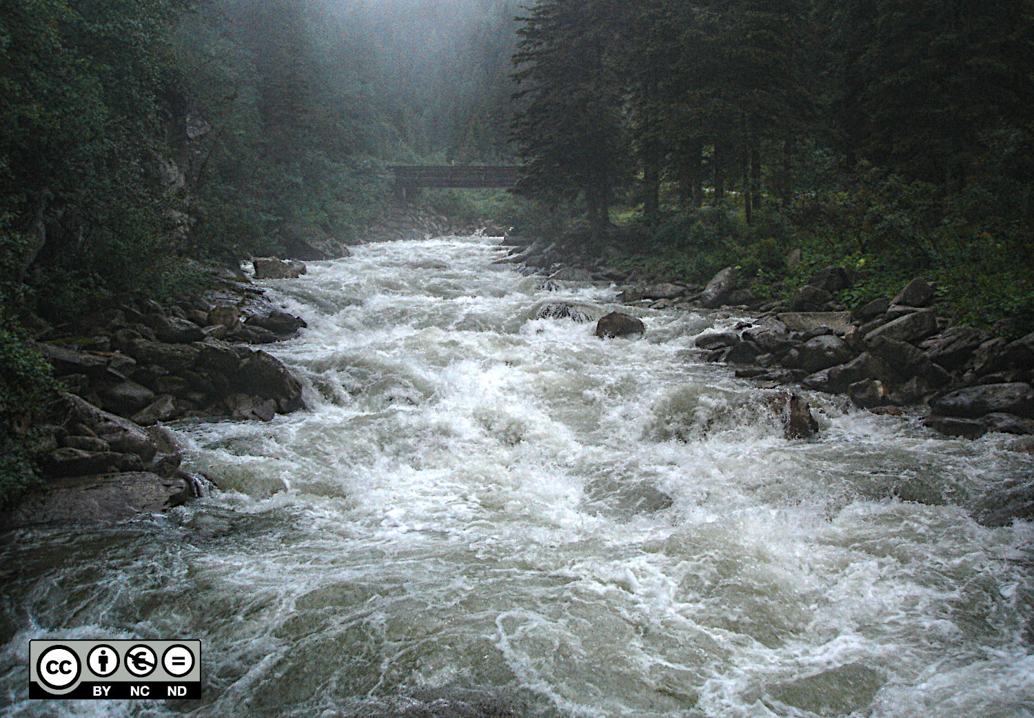
Figure 2:The Krimmler Ache in Austria during a small flood event. Even though the watershed has a high Feststoffeintrag, the transport capacity of the water in this river section is so high that the riverbed predominantly consists of large boulders. Thus, the river section can be characterized as naturally sediment supply-limited (picture: Sebastian Schwindt 2010).
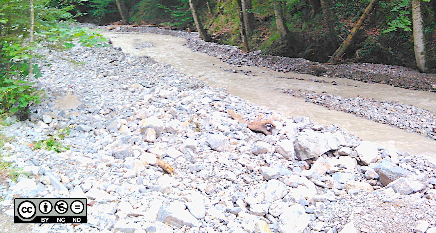
Figure 3:Der Jenbach in den Bayerischen Alpen (Deutschland) nach einer intensiven natürlichen Sedimentversorgung in stromaufwärts gelegener Reichweite in Form eines Erdrutsches. Der Flussabschnitt kann als transportkapazitätsbegrenzt charakterisiert werden (Bild: Sebastian Schwindt 2020).
Warum ist die Unterscheidung zwischen Sedimentversorgung und transportkapazitätsbegrenzten Flüssen für die numerische Modellierung wichtig?
Gaia provides different formulae for calculating bedload transport, which are partially either derived from lab experiments with infinite sediment supply (e.g., the Meyer-Peter & Müller (1948) formula and its derivates, see below) or from field measurements in partially transport capacity-limited rivers (e.g., Wilcock (1993)). Formulae that account for limited sediment supply often involve a correction factor for the Shields parameter.
Formeln und Parameter
Geschiebe is typically designated with (in kgsm i.e. weight per unit time and width) and accounts for particulate transport in the form of the displacement of rolling, sliding, and/or jumping coarse particles. In river hydraulics, the so-called Dimensionslose Schubspannung, also referred to as Shields parameter Shields, 1936, is often used as a threshold value for the mobilization of sediment from the riverbed. TELEMAC and Gaia build on a dimensionless expression of bedload transport intensity according to Einstein (1950):
where is the density of sediment grains; is the ratio of sediment grain and water density (typically 2.68) Schwindt, 2017; is gravitational acceleration; and is the characteristic grain diameter of the sediment class (cf. Sedimentklassen). Note that the dimensionless expression and the dimensional expression represent unit bedload (i.e., bedload normalized by a unit of width). Gaia outputs are dimensional and correspond to (recall the VARIABLES FOR GRAPHIC PRINTOUTS definitions in the General Parameters section) where the unit of width corresponds to the edge length of a numerical mesh cell over which the mass fluxes are calculated.
Comment on the Original Einstein (1950) Expression
The original equation for can be found on page 34 (Equation 42) in Einstein (1950). This formula involves an additional division by the gravitational acceleration , which does not appear in later references to the Einstein expression of and would also not result in a dimensionless term. For this reason, Equation (1) is adapted here.
Equation (1) expresses only the dimensional conversion for bedload transport (i.e., the way how dimensions are removed or added to sediment transport). In fact, this is only the first step to solve the other side of a bedload equation using a (semi-) empirical formula. To calculate , Gaia provides a set of (semi-) empirical formulae, which can be modified with user Fortran files and defined in the Gaia steering file with the BED-LOAD TRANSPORT FORMULA FOR ALL SANDS integer keyword. Table 1 lists possible integers for the keyword to define a bedload transport formulae, including references to original publications, formula application ranges, and the names of the Fortran source files for modifications.
Table 1:Bedload transport formulae implemented in Gaia with application limits regarding the grain diameter , cross section-averaged Froude number , slope , water depth , and flow velocity . The Fortran files live in the /telemac/sources/gaia/ directory.
| Gaia | Author(s) | Fr; ; ; and | User Fortran | |
|---|---|---|---|---|
| (no.) | (ref.) | (10m) | (-); (-); (m); (m/s) | (file name) |
1 | Meyer-Peter & Müller (1948) | 0.4 28.6 | 10639 0.00040.02 0.011.2 0.2 | bedload_meyer.f |
2 | Einstein (1950)-Brown (1949) | 0.2532 | bedload_einst.f | |
3 | Engelund & Hansen (1967) + Chollet & Cunge (1979) | 0.155.0 | 0.110 | bedload_engel_cc.f |
7 | Van Rijn (1984) | 0.62.0 | 0.5 0.2 | bedload_vanrijn.f |
10 | Wilcock & Crowe (2003) | 0.063 | bedload_wilcock_crowe.f | |
30 | Engelund & Hansen (1967) | 0.155.0 | 0.110 | bedload_engel.f |
Beachten Sie, dass die Engelund-Hansen-Formeln (Optionen 3 und 30) den gesamten Sedimenttransport berechnen, dh die Summe aus Geschiebefracht und Schwebstofffracht. Wenn Sie also diese Formeln verwenden, aktivieren Sie nicht zusätzlich die Modellierung der Schwebstofffracht, um Doppelzählungen zu vermeiden.
Um die Formel Meyer-Peter & Müller (1948) (1 gemäß Tab. 1) in diesem Tutorial zu verwenden, fügen Sie die folgende Zeile zur Steuerungsdatei gaia-morphdynamics.cas hinzu:
/ continued: gaia-morphodynamics.cas
/
/ BEDLOAD
/
BED LOAD FOR ALL SANDS : YES / deactivate with NO
BED-LOAD TRANSPORT FORMULA FOR ALL SANDS : 1
The following sections provide more details on how is calculated with the pre-defined formulae listed in Tab. 1.
User Fortran Files
To implement a user Fortran file, copy the original TELEMAC Fortran file from the /telemac/sources/ directory (e.g., /telemac/sources/gaia/bedload_einst.f) to the project directory (e.g., /telemac/simulations/gaia-tutorial/user_fortran/bedload_einst.f). Finally, tell TELEMAC where to look for user fortran files by defining the following keyword in a steering file (e.g., in gaia-morphodynamics.cas):
FORTRAN FILE : 'user_fortran'
Meyer-Peter und Müller (1948)
The Meyer-Peter & Müller (1948) formula was published in 1948 by Swiss researchers Eugen Meyer-Peter, professor at ETH Zurich and founder of the school’s hydraulics laboratory (Zurich’s famous VAW), and Robert Müller. Their empirical formula is the result of more than a decade of collaboration and the elaboration began one year after the VAW was founded in 1931 when Robert Müller was appointed assistant to Eugen Meyer-Peter. The two scientists also worked with Henry Favre and Hans-Albert Einstein who came up with another approach for calculating bedload. An early version of the Meyer-Peter & Müller (1948) formula was published in 1934 and it is the basis for many other formulas that refer to a critical Dimensionslose Schubspannung (i.e., Shields parameter). It is important to remember that the formula is based on data from lab flume experiments with high sediment supply. This is why bedload transport calculated with the Meyer-Peter & Müller (1948) formula corresponds to the hydraulic transport capacity of an alluvial channel. Thus, the Meyer-Peter & Müller (1948) formula tends to overestimate bedload transport and it is inherently designed for estimating bedload based on simplified 1d cross section-averaged hydraulics (see also the Python sediment transport exercise). Good results can be expected when flood flows are simulated in an alluvial river section.
Letztendlich kann die linke Seite von Gleichung (1) () mit der Meyer-Peter & Müller (1948)-Formel wie folgt berechnet werden:
Wobei der MPM-Koeffizient ist (Standard ist 8), bezeichnet den Shields parameter ( 0.047 und bis zu 0.07 in Bergflüssen), und ist der Dimensionslose Schubspannung. Bei Verwendung der Meyer-Peter & Müller (1948)-Formel mit Gaia wird die Konsistenz mit den Originalpublikationen sichergestellt, indem und in der Steuerungsdatei** definiert werden:
/ continued: gaia-morphodynamics.cas
/
/ BEDLOAD
BED-LOAD TRANSPORT FORMULA FOR ALL SANDS : 1 / see above
CLASSES SHIELDS PARAMETERS : 0.047;0.047;0.047
MPM COEFFICIENT : 8To directly continue with the tutorial using the Meyer-Peter & Müller (1948) formula, jump to the correction factors section.
Einstein-Brown (1942/49)
Hans Albert Einstein, Sohn des berühmten Albert Einstein, war ein Pionier der Wahrscheinlichkeitsanalysen des Sedimenttransports. Insbesondere stellte er die Hypothese auf, dass der Beginn und das Ende der Sedimentbewegung in Bezug auf Wahrscheinlichkeiten ausgedrückt werden können. Darüber hinaus nahm Einstein an, dass die Sedimentbewegung eine Reihe von schrittweisen Verschiebungen ist, gefolgt von Ruheperioden, und dass der durchschnittliche Abstand einer Partikelverschiebung etwa das Hundertfache des Teilchendurchmessers beträgt. Um die Beobachtungen zu berücksichtigen, die er in Laborflimmerexperimenten gemacht hat, führte Einstein außerdem das Verstecken und Heben von Korrekturkoeffizienten ein Einstein, 1942.
Die Einstein-Formel unterscheidet sich von jeder Meyer-Peter & Müller (1948)-basierten Formel dadurch, dass sie keine Schwelle für die beginnende Bewegung von Sedimenten impliziert. Trotz oder weil Einsteins Sedimenttransporttheorie komplexer ist als viele andere Geschiebetransportformeln, wurde sie in technischen Anwendungen nicht sehr populär. Heute ermöglicht Gaia die benutzerfreundliche Anwendung von Einsteins Formel, die 1949 von Brown (1949) auf einer hydraulischen Konferenz vorgestellt wurde. Laut Einstein (1942)-Brown (1949) wird die linke Seite von Gleichung (1) () wie folgt berechnet:
wo
ist der dimensionslose Teilchendurchmesser berechnet als:
Dabei ist das Verhältnis von Sedimentkorn und Wasserdichte (normalerweise 2,68); ist die Gravitationsbeschleunigung; und ist die kinematische Viskosität von Wasser (10ms@s) Schwindt, 2017.
Um die Einstein (1942)-@-Brown (1949) Formeln in Gaia zu verwenden, verwenden Sie:
BED-LOAD TRANSPORT FORMULA FOR ALL SANDS : 2Engelund-Hansen (1967) / Chollet-Cunge
The Engelund & Hansen (1967) formula accounts for total sediment transport including Geschiebe and Schwebstoff. Starting from the Bagnold power-approach Bagnold, 1966Bagnold, 1980, the Engelund & Hansen (1967) formula was developed for sediment transport calculations over dune channel beds. The approach accounts for energy losses required to drive particles uphill on dunes of the riverbed. The Bagnold (1966) theory considers the total shear as the sum of the shear transmitted between grains and the fluid, and the shear transmitted by momentum changes caused by intergranular collisions. Thus, erosion takes place as long as the Dimensionslose Schubspannung is greater or equal to its critical value (i.e., the Shields parameter). Gaia implements the Engelund & Hansen (1967) by calculating the left side of Equation (1) () as follows:
where is an adimensional friction coefficient and is the Shields number without the skin friction correction factor. Read more about skin friction in the correction factors section. To use the original Engelund & Hansen (1967) formula in Gaia use:
BED-LOAD TRANSPORT FORMULA FOR ALL SANDS : 30Darüber hinaus hat Chollet & Cunge (1979) eine schrittweise Funktion zur Berechnung eines modifizierten Shields-Parameters eingeführt, der verschiedene Transportregime berücksichtigt:
To apply the Chollet & Cunge (1979) modification of the Engelund & Hansen (1967) formula use:
BED-LOAD TRANSPORT FORMULA FOR ALL SANDS : 3van Rijn (1984)
Die Sedimenttransportformel von Leo van Rijn Van Rijn, 1984 ist inspiriert von den Theorien von Bagnold (1980), Einstein (1942) und Ackers & White (1973). Die Van Rijn (1984)-Formeln gehen davon aus, dass die Geschiebefracht von der Schwerkraft dominiert wird, während der Transport der Schwebstofffracht gemäß Bagnold (1980) durch Turbulenzen gesteuert wird. Zu diesem Zweck berechnen die Van Rijn (1984) Formeln den Geschiebetransport ähnlich wie Ackers & White (1973), wo die Transportraten von Reibungsgeschwindigkeiten abhängen. Um sein bettnahes Feststofftransportmodell zu kalibrieren, verwendete Van Rijn (1984) Daten aus Experimenten an Flachbettkanälen mit einem durchschnittlichen Sedimentkorndurchmesser von 1,8 mm. Van Rijn (1984) führte zusätzliche Experimente durch, um die Ergebnisse seines Modells gegen unterschiedliche Korndurchmesser zwischen 0,2 und 2 mm zu überprüfen. Darüber hinaus hat Van Rijn (1984) Kriterien für Sedimentsuspension basierend auf Laborexperimenten mit Korndurchmessern von weniger als 0,5 mm und durch empirische Vereinfachung der Kalibrierparameter festgelegt. Während die ursprüngliche Van Rijn (1984)-Formel den gesamten Sedimenttransport berücksichtigt (d.h. Geschiebe und Schwebstoff), sind die folgenden Erklärungen für die Implementierung in Gaia nur auf Geschiebe beschränkt.
Laut Van Rijn (1984) wird die linke Seite von Gleichung (1) () wie folgt berechnet:
Explanations of the Dimensionslose Schubspannung , its critical value (i.e., the Shields parameter), and the dimensionless grain diameter are provided in the above sections on the Meyer-Peter and Müller and the Einstein-Brown formulae.
To use the Van Rijn (1984) formula in Gaia use:
BED-LOAD TRANSPORT FORMULA FOR ALL SANDS : 7Wilcock-Crowe (2003)
Der Wilcock & Crowe (2003)-Ansatz ist ein Multifraktions-Sedimenttransportmodell, das hauptsächlich in gepanzerten Flussabschnitten zur Modellierung der Aggradation oder Degradation von Betten angewendet wird. Das Modell basiert auf Oberflächenuntersuchungen und ist besonders für die Vorhersage von transienten Bedingungen der Bettpanzerung geeignet. Es berücksichtigt die volle Größenverteilung der Bettoberfläche (vom feinsten Sand bis zum gröbsten Kies) und wurde mit insgesamt 49 Flume-Experimenten mit kleinen bis hohen Wasserableitungen und fünf verschiedenen Sedimentmischungen kalibriert.
The approach takes up the idea of Parker (1990) on applying a reference shear stress at which little but constant solid transport rate can be observed. The reference shear stress is close to, but a little bit larger than the Shields parameter . To this end, Wilcock & Crowe (2003) implement a reference transport rate of 0.002 as proposed by Parker (1990).
Moreover, the multi-fraction Wilcock & Crowe (2003) model uses the complete sediment grain size distribution of the riverbed surface and calculates bedload transport for each of the specified grain size classes. The sediment transport model builds on flume experiments from Proffitt & Sutherland (1983) and Parker (1990), and it accounts for hiding/exposure effects on gravel transport as a function of the sand fraction in the riverbed. The hiding-exposure function is designed to resolve discrepancies observed from previous experiments, including the hiding-exposure effect of sand content on gravel transport for weak to high values of sand content in the bulk.
Kurz gesagt stellt das Wilcock & Crowe (2003)-Modell eine Weiterentwicklung der Meyer-Peter & Müller (1948)-Formel dar, greift die Implementierung einer Referenztransportrate Parker, 1990 auf und ist auf Versteck-/Expositionseffekte als Funktion des Sandanteils kalibriert.
Um die Formel Wilcock & Crowe (2003) in Gaia zu verwenden, definieren Sie mehrere sediment classes und verwenden Sie:
BED-LOAD TRANSPORT FORMULA FOR ALL SANDS : 10Korrekturfaktoren
Korrekturfaktoren für den Sedimenttransport können erforderlich sein, um die transversale Kanalsteigung, Sekundärströme oder die Korrektur der Hautreibung zu berücksichtigen.
Reibungskorrektureinrichtungen
Reibung wird oft mit vereinfachten Ansätzen betrachtet, die Hautreibung und Formwiderstand in einen Topf werfen, aber in einem zweidimensionalen Modell beeinflusst nur die Hautreibung die Geschiebefracht. Einstein (1950) berücksichtigt Hautreibung mit einem Korrekturfaktor für (dimensionale) Bettscherbeanspruchung :
Der Korrekturfaktor ist definiert als das Verhältnis des reinen Hautreibungskoeffizienten und des globalen Reibungskoeffizienten (d.h. stückige Hautreibung und Formwiderstand):
Der reine Hautreibungskoeffizient wird wie folgt berechnet:
wobei die Von Karmàn (1930)-Konstante (0.4) ist, die Wassertiefe ist und die repräsentative Rauheitslänge ist, die als berechnet wird, wobei ein Kalibrierungsparameter ist (lesen Sie mehr im Abschnitt über bedload calibration).
Gaia verwendet standardmäßig den Korrekturkoeffizienten der Hautreibung, den sie vom hydrodynamischen Solver ableitet (d. H. Telemac2d/3d). In sehr flachen Gewässern kann dieses Verhalten zu Instabilitäten führen. Daher kann das Schlüsselwort SKIN FRICTION CORRECTION in Gaia festgelegt werden, um die Korrekturfaktorberechnung zu steuern:
0: Deaktiviert Korrektur, Einstellung (Gesamtbettscherspannung von Hydrodynamik wird direkt verwendet)1: Ermöglicht die Korrektur der Hautreibung (Standard), berechnet gemäß Gleichungen (10) und (11)2: Ermöglicht einen Bettform-Prädiktor, der Wellen bei der Berechnung berücksichtigt
To disable skin friction correction (i.e., set to 1), add the following to the Gaia steering file (not used in this tutorial):
SKIN FRICTION CORRECTION : 0 / default is 1 to enable skin friction correctionDer Koeffizient (Verhältnis zwischen Hautreibungsrauhigkeit und mittlerem Durchmesser) kann mit dem Schlüsselwort RATIO BETWEEN SKIN FRICTION AND MEAN DIAMETER geändert werden (Standard ist 3.0). Lesen Sie mehr in Abschnitt 3.1.8 des Gaia manual].
The finer the sediment of the riverbed, the more important turbulence created by the bed shape becomes. For instance, skin friction calculated based on a multiple of the diameter of a sand grain’s characteristic roughness length is very small. However, sand tends to shape the riverbed into ripple or dune forms, which cause additional bedform turbulence, as featured in the video below.
by Sebastian Schwindt@ Hydro-Morphodynamics channel on YouTube.
Standardmäßig berücksichtigt Gaia keine Turbulenzen (d. H. Rauheitseffekte) von Bettformen, aber es kann aktiviert werden, indem das Schlüsselwort COMPUTE BED ROUGHNESS AT SEDIMENT SCALE** auf YES gesetzt wird (Standard ist NO). Dann kann eine der folgenden Optionen für das Schlüsselwort BED ROUGHNESS PREDICTOR OPTION definiert werden:
1für eine Flachbettannahme mit dem Standardansatz von (geändert mit RATIO BETWEEN SKIN FRICTION AND MEAN DIAMETER).2for ripple bedforms. For currents only, the ripple roughness is a function of the mobility number. For waves and combined waves-currents, bedform dimensions are calculated as a function of wave parameters following Wiberg & Harris (1994).3für Van Rijn (2007) Gesamtbettrauheit Prädiktor (nur Ströme). Die Gesamtrauhigkeit wird zerlegt in Kornrauhigkeit, kleinräumige Rillenrauhigkeit, Mega-Ripple-Komponente und Dünenrauhigkeit.
Das Gaia manual] (Abschnitt 3.1.9) fasst den Satz von Gleichungen zusammen, die in die Berechnung der ** BED ROUGHNESS PREDICTOR OPTION** eingehen.
Richtung und Größe (Intensität)
Natural rivers are characterized by non-straight lines of the Talweg, which involves that water and sediment are subjected to curve effects. However, water and sediment behave differently in a curve because sediment has greater inertia than water Mosselman & Le, 2016. Gaia accounts for the inertia of sediment transport as a function of water depth, curve radius, a spiral flow coefficient (A), and the depth-averaged, 2d velocities U and V. In addition, sediment transport reacts more inert to horizontal (transversal) channel slope and can be considered in and directions (see also the explanation of the Exner-Gleichung). To this end, Gaia calculates the slope-corrected unit bedload transport as follows:
Hierbei ist der Winkel zwischen der Längsachse () und dem Geschiebetransportvektor (siehe auch Exner-Gleichung), ist ein empirischer Geschiebeintensitätskorrekturfaktor von Koch & Flokstra (1980) und ist die Flussbetthöhe.
Der Grad der Geschiebeabweichung (über ) und der -Faktor können in Gaia mit den Schlüsselwörtern FORMULA FOR DEVIATION und FORMULA FOR SLOPE EFFECT (horizontal) definiert werden. Um eines oder beide Keywords zu verwenden, muss das Schlüsselwort SLOPE EFFECT auf YES gesetzt werden (Standard ist YES).
Das Schlüsselwort FORMULA FOR DEVIATION kann die folgenden ganzzahligen Werte verwenden, um eine bestimmte Formel für die Funktion Sedimentform zu definieren (siehe Abschnitt 3.1.4 in Gaia manual]):
1für Bett-Level-Berechnung gemäß Koch & Flokstra (1980) (Standard).2for the Talmon et al. (1995) approach based on laboratory experiments, which should be used with the PARAMETER FOR DEVIATION keyword for setting theBETA2parameter (its default isPARAMETER FOR DEVIATION : 0.85, but an optimum was found with1.6Mendoza et al., 2017).3für den Apsley & Stansby (2008)-Ansatz basierend auf dem kritischen Shields-Parameter und dem Reibungswinkel des Sediments, der mit dem Schlüsselwort FRICTION ANGLE OF THE SEDIMENT verwendet werden sollte (Standard ist40.).
Das Schlüsselwort FORMULA FOR SLOPE EFFECT beeinflusst nicht nur die Richtung des Sedimenttransports, sondern auch die Größe (oder Intensität) der Geschiebefracht und kann folgende Werte annehmen:
1für Bett-Level-Berechnung gemäß Koch & Flokstra (1980) (Standard und ähnlich wie FORMULA FOR DEVIATION). Die Einstellung1ermöglicht die Definition des empirischen Korrekturfaktors der Bettneigung in Gleichung (12) durch das Schlüsselwort BETA (Standard istBETA : 1.3).Um die Änderung der Betthöhe zu erhöhen, erhöhen Sie ** BETA **.
Um die Änderung der Betthöhe zu verringern, verringern Sie ** BETA **.
2für die Hangkorrektur in Sandbettflüssen basierend auf einem Ansatz von Soulsby (1997), der eine Korrektur des Shields parameter als Funktion des Reibungswinkels des Sediments und des Flussbetthangs anwendet. Der Reibungswinkel kann mit dem zusätzlichen Schlüsselwort FRICTION ANGLE OF THE SEDIMENT definiert werden (Standard ist40.).3für den Apsley & Stansby (2008)-Ansatz, der sowohl den kritischen Shields-Parameter als auch die effektive dimensionslose Scherspannung modifiziert. Verwenden Sie mit dem Schlüsselwort FRICTION ANGLE OF THE SEDIMENT.
Sekundärströme
Secondary currents may occur in curved channels (i.e., in most near-census natural rivers) where water moves like a gyroscope through river bends. More specifically, secondary flows are helical motions in which water near the surface is driven toward the outer bend, while water near the riverbed is driven toward the inner bend. Thus, secondary flows are a 3d phenomenon that can be represented in 2d models only with auxiliary approaches. For Geschiebe transport, the near-bed current toward the inner bend is especially important, because it promotes erosion at the outer bend and may lead to deposition at the inner bend.
By default, Telemac2d and Gaia do not consider secondary currents, but an approach based on Engelund (1974) can be enabled by setting the SECONDARY CURRENTS keyword to YES (default is NO). In Gaia, the spiral flow coefficient is set to 7 (Engelund’s value). The SECONDARY CURRENTS ALPHA COEFFICIENT keyword can be used to modify this coefficient as a function of channel bottom roughness:
SECONDARY CURRENTS ALPHA COEFFICIENT : 0.75für ein sehr raues FlussbettSECONDARY CURRENTS ALPHA COEFFICIENT : 1.0für ein glattes Flussbett (Standard)
Für dieses Tutorial verwenden:
/ continued: gaia-morphodynamics.cas
/ ...
SECONDARY CURRENTS : YES
SECONDARY CURRENTS ALPHA COEFFICIENT : 0.8Grenzbedingungen
The Gaia Basis section on boundary conditions explains the geometric definition of open liquid boundaries in the *.cli files. To prescribe a bedload transport of 10 kgs (total solid discharge without pores) across the upstream (LIEBOR=5) boundary and free outflow at the downstream (LIEBOR=4) boundary, add the PRESCRIBED SOLID DISCHARGES keyword to the Gaia steering file (gaia-morphodynamics.cas):
/ continued: gaia-morphodynamics.cas
/ ...
PRESCRIBED SOLID DISCHARGES : 10.;0.
Recall that the first and second values in the list of prescribed solid discharges refer to the first and second open boundary listed in the boundaries-gaia.cli, respectively (i.e., upstream and downstream in that order).
Gaia can be run with liquid boundary files for assigning time-dependent solid discharges (the outflow should be kept in equilibrium). Solid discharge time series can be implemented using 455-5 boundary definitions, analogous to the descriptions of the Telemac2d unsteady boundary setup. For more guidance, have a look at the yen-2d example (telemac/examples/gaia/yen-2d) featuring a quasi-steady bedload simulation at the Rhine River. In addition, more background information about the definition of bedload boundary conditions can be found in sections 3.1.10-3.1.12 in the Gaia manual.
Beispielanträge
Examples for the implementation of bedload come along with the TELEMAC installation (in the /telemac/examples/gaia/ directory). The following examples in the gaia/ folder feature (pure) bedload calculations:
Anwendung des Wilcock-Crowe formula (mehrere Sedimentklassen): wilcock crowe-t2d/
Geschiebefracht in einem Bogen des Rheins mit quasi stetigen (unruhigen) Strömungsverhältnissen: yen-2d/
Geschiebe gekoppelt mit Telemac3d: bosse-t3d/
Modell eines gepanzerten (schichteten) Flussbettes: guenter-t2d/
Küstensandtransport in Verbindung mit dem Wellenausbreitungsmodul Tomawac: littoral-t2d-tom/
Kupplung mit dem Baggermodul Nestor: nestor dig test-t2d/
Finite Volume Solver mit zeitabhängiger Feststoffentladung in einem
*.liq: flume bc-t2d/
- Church, M., & Ferguson, R. I. (2015). Morphodynamics: Rivers beyond steady state. Water Resources Research, 51, 1883–1897. 10.1002/2014WR016862
- Meyer-Peter, E., & Müller, R. (1948). Formulas for Bed-Load transport. IAHSR, Appendix 2, 2nd meeting, 39–65. http://resolver.tudelft.nl/uuid:4fda9b61-be28-4703-ab06-43cdc2a21bd7
- Wilcock, P. (1993). Critical shear stress of natural sediments. Journal of Hydraulic Engineering, 119, 491–505.
- Shields, A. (1936). Anwendung der Ähnlichkeitsmechanik und der Turbulenzforschung auf die Geschiebebewegung [Application of the similarity in mechanics and turbulence research on the mobility of bed load] (Vol. 26). Preußische Versuchsanstalt für Wasserbau und Schiffbau. http://resolver.tudelft.nl/uuid:61a19716-a994-4942-9906-f680eb9952d6
- Einstein, H. A. (1950). The Bed-Load Function for Sediment Transport in Open Channel Flows. Technical Bulletin of the USDA Soil Conservation Service, 1026, 71. 10.22004/ag.econ.156389
- Schwindt, S. (2017). Hydro-morphological processes through permeable sediment traps [Thesis No. 7655, Laboratory of Hydraulic Constructions (LCH), Ecole Polytechnique fédérale de Lausanne (EPFL)]. 10.5075/epfl-thesis-7655
- Brown, C. B. (1949). Sediment Transport. In H. Rouse (Ed.), Engineering hydraulics: proceedings of the fourth Hydraulics conference, June 12-15, 1949. John Wiley. https://www.worldcat.org/title/engineering-hydraulics-proceedings-of-the-fourth-hydraulics-conference-iowa-institute-of-hydraulic-research-june-12-15-1949/oclc/802562429
- Engelund, F., & Hansen, E. (1967). A monograph on sediment transport in alluvial streams. TEKNISKFORLAG Skelbrekgade 4 Copenhagen V, Denmark.
- Chollet, J. P., & Cunge, J. A. (1979). New Interpretation of Some Head Loss-Flow Velocity Relationships for Deformable Movable Beds. Journal of Hydraulic Research, 17(1), 1–13. 10.1080/00221687909499596
- Van Rijn, L. C. (1984). Sediment Transport, Part I: Bed Load Transport. Journal of Hydraulic Engineering, 110(10), 1431–1456. 10.1061/(ASCE)0733-9429(1984)110:10(1431)
- Wilcock, P. R., & Crowe, J. C. (2003). Surface-based Transport Model for Mixed-Size Sediment. Journal of Hydraulic Engineering, 129(2), 120–128. 10.1061/(ASCE)0733-9429(2003)129:2(120)
- Wong, M., & Parker, G. (2006). Reanalysis and Correction of Bed-Load Relation of Meyer-Peter and Müller Using Their Own Database. Journal of Hydraulic Engineering, 132(11), 1159–1168. 10.1061/(ASCE)0733-9429(2006)132:11(1159)
- Einstein, H. A. (1942). Formulas for the Transportation of Bed Load. Transactions of the American Society of Civil Engineers, 107(1), 561–577.
- Bagnold, R. A. (1966). An Approach to the Sediment Transport Problem from General Physics. In Geological Survey Professional Paper 422-I. U.S. Government.
- Bagnold, R. A. (1980). An empirical correlation of bedload transport rates in flume and natural rivers. Proceedings of the Royal Society of London, A(372), 453–473. 10.1098/rspa.1980.0122