Erste Schritte
The steady 2d tutorial hypothesizes that the discharge of a river is constant over time. However, the discharge of a river is never truly constant (i.e., never steady) and varies slightly from second to second, even in controlled rivers. To model the inherently unsteady flows of rivers, we can discretize time-dependent discharge (e.g., a flood hydrograph) in a numerical model as a series of steady discharges. Figure 1 illustrates the discretization of a natural flood hydrograph into steps of steady flows, which will be used in this chapter. Note that the hydrograph starts at Time = 15000, which is the result of the dry-initialized steady2d simulation.
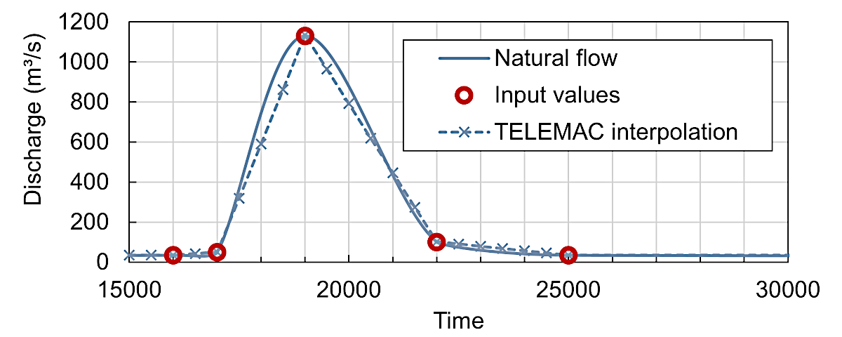
Figure 1:Die Diskretisierung eines kontinuierlichen Hydrographen in Stufen stetiger Strömungen (qualitativer Hydrograph für dieses Tutorial).
This chapter features the implementation of a quasi-steady discharge hydrograph into a hydrodynamic Telemac2d simulation through the definition of an inflow sequence (red circles in Fig. 1). The tutorial builds on the steady simulation of a discharge of 35 m/s and requires the following data from the pre-processing and steady2d tutorials, which can be downloaded by clicking on the filenames:
Die Computational Mesh qgismesh.slf Datei (verwendet EPSG:32633 - ETRS 89 / UTM Zone 33N).
Die Randdefinitionen boundaries.cli Datei].
Die Ergebnisdatei r2dsteady.slf] des dry initialized steady 2d simulation endet bei
t=15000für 35 m/s.
Consider saving the files in a new folder, such as /unsteady2d-tutorial/.
Modellanpassungen
Die Implementierung von instationären Flüssen erfordert die Anpassung von Schlüsselwörtern und zusätzlichen Schlüsselwörtern (z. B. zur Verknüpfung von Flüssigkeitsranddateien) in der Steuerungsdatei (.cas) aus dem steady2d-Tutorial (Download steady2d.cas].
Erste Bedingungen von Hotstart
Die folgenden Beschreibungen beziehen sich auf Abschnitt 4.1.3 im Telemac2d Manual.]
To speed up the calculations and provide a well-converging baseline for the quasi-steady calculations, this tutorial re-uses the output of the steady 2d simulation with dry initial conditions (see the Ursprüngliche Bedingungen section). This type of model initialization is also called hotstart. To hotstart the simulation, the steady results file r2dsteady.slf needs to be defined as PREVIOUS COMPUTATION FILE:
COMPUTATION CONTINUED : YES
PREVIOUS COMPUTATION FILE : r2dsteady.slf / results of 35 CMS steady simulation
/ INITIAL TIME SET TO ZERO : 0 / avoid restarting at 15000
An INITIAL TIME SET TO ZERO keyword may be defined to reset the time from the previous computation file from 15000 to 0. However, this tutorial does not use this option and continues at timestep 15000.
Um mehrdeutige Definitionen von Anfangsbedingungen zu vermeiden, deaktivieren Sie ** (d.h. löschen oder kommentieren Sie Zeilen mit einem /) das Schlüsselwort **INITIAL BEDINGUNGEN **:
/ INITIAL CONDITIONS : 'ZERO DEPTH'Allgemeine Parameter
To simulate the hydrograph shown in Fig. 1, the simulation must run for at least another 15000 time steps (i.e., from t=15000 to t=30000). Since printing out (intermediate) results has a significant effect on computing time, increase the graphic printout timestep to 500 (i.e., decrease the printout frequency compared to 200 used for the steady simulation):
TIME STEP : 1.
NUMBER OF TIME STEPS : 15000
GRAPHIC PRINTOUT PERIOD : 500
LISTING PRINTOUT PERIOD : 500
Offene Grenzen
This section features the implementation of quasi-steady (unsteady) flow conditions at the open liquid boundaries with a time-dependent inflow hydrograph and a downstream Wasserstands-Abfluss Beziehung (recall the rationales behind the choice of boundary types from the pre-processing tutorial).
** Definieren Sie einen Quasi-steady Hydrographen **
With the dry-initialized model ending at =15000, the hydrograph needs to start at 15000, even though the model start will represent time zero of the unsteady simulation. To implement the triangular-shaped hydrograph shown in Fig. 1, create a new file called inflows.liq in the simulation folder. Open the new inflows.liq file in a text editor and add the red-circled points in Fig. 1 as time-dependent flow information at the upstream (1) and downstream (2) open (liquid) boundaries. In this file:
Add a file header starting with
#signs (commented lines ignored by TELEMAC).Implementieren Sie 2 Spalten für die Zeit T () und die Upstream-Zuflussrate Q(1).
Trennen Sie die Spalten mit spaces.
The first column must be time
Twith strictly monotonously increasing values and the last time value must be greater than or equal to the last simulation timestep.
Daher sollte die Datei inflows.liq] ähnlich aussehen:
# Inflow hydrograph
#
T	Q(1)
s	m3/s
15000	35
16000	35
17000	50
19000	1130
22000	101
25000	35
99000	35
Die ursprüngliche Datei boundaries.cli beschreibt die nachgelagerte Grenze mit * prescribed Q und H* (Typ 5 5 5). In der instationären Berechnung muss Q jedoch frei sein (sonst muss Q(2) in inflows.liq mit einer zusätzlichen Spalte definiert werden) und aus diesem Grund erfordert die boundaries.cli-Datei einige Anpassungen:
** Öffnen Sie die bereitgestellte boundaries.cli Datei mit einem Texteditor (z. B. NotepadPlus (Texteditor) unter Windows).
Use find-and-replace (e.g.,
CTRL+Hkeys in Notepad++, orCTRL+Fkeys in other text editors):Find
5 5 5Ersetzen mit
4 5 5Klicken Sie auf Ersetzen alle Upstream-Grenzknoten.
** Speichern Sie die Datei als **boundaries-unsteady.cli ** und schließen Sie sie.
Um die richtigen Einstellungen zu überprüfen download borders-unsteady.cli für die unstetige Simulation].
Passen Sie in der Steering-Datei den Dateinamen für die Randbedingungen an und fügen Sie den Link zu inflows.liq hinzu:
BOUNDARY CONDITIONS FILE : boundaries-unsteady.cli
/ ...
LIQUID BOUNDARIES FILE : inflows.liq
Ratingkurve (Stage-Discharge-Relation) Um die Verwendung eines Wasserstands-Abfluss Beziehung für eine offene (liquide) Grenze zu aktivieren, muss das Schlüsselwort STAGE-DISCHARGE CURVES zur Steuerungsdatei hinzugefügt werden. Dieses Keyword erfordert eine Liste bestehend aus den folgenden Ganzzahlen:
0ist der Standard, der die Verwendung einer Bühnenentladungskurve deaktiviert.1applies prescribed elevations as a function of calculated flow rate (discharge).2applies prescribed flow rates (discharge) as a function of calculated elevation.
Das Schlüsselwort STAGE-DISCHARGE CURVES ist eine Liste, die eine der drei Ganzzahlen (d.h. entweder 0, 1 oder 2) den offenen (liquiden) Grenzen zuweist. In diesem Tutorial aktiviert die Einstellung STAGE-DISCHARGE CURVES : 0;1 die Verwendung eines Wasserstands-Abfluss Beziehung für die nachgelagerte Grenze nur dann, wenn die upstream offene Grenze Nummer 1 auf 0 und die downstream offene Grenze Nummer 1 auf 0 gesetzt ist.
The form (curve) of the Wasserstands-Abfluss Beziehung needs to be defined in a stage-discharge file (ASCII text format). Such files typically apply to the downstream boundary of a model at control sections (e.g., a free overflow weir). This tutorial uses the following relationship that is stored in a file called ratingcurve.txt (download):
# Downstream ratingcurve.txt
#
Z(2)	Q(2)
m	m3/s
371.33	35
371.45	50
371.86	101
375.73	1130
379.08	2560
How to assign different stage-discharge curves at multiple boundaries?
To define Wasserstands-Abfluss Beziehungs at multiple open boundaries (e.g., at river diversions or tributaries), add the curves to the same file. TELEMAC automatically recognizes where the curves apply by the number given in parentheses after the parameter name in the column header. For instance, in the above example for this tutorial, the column headers Z(2) and Q(2) tell TELEMAC to use these values for the second (i.e., here, the downstream) open boundary. The column order is not important because TELEMAC reads the curve type (i.e., either or ) from the STAGE-DISCHARGE CURVES keyword.
The following file block would prescribe Wasserstands-Abfluss Beziehungs to the upstream and downstream boundary conditions in this tutorial. However, the file cannot be used here unless the upstream boundary type is changed to 5 5 5 (prescribed H and Q) in the boundaries.cli file (read more in the pre-processing tutorial).
#
# Downstream Rating Curve
#
Z(2)	Q(2)
m	m3/s
371.33	35
371.45	50
371.86	101
375.73	1130
379.08	2560
#
# Upstream Rating Curve
#
Q(1)  Z(1)
m3/s  m
35    371.33
50    371.45
101   371.86
1130  375.73
2560  379.08
Um die Stage-Discharge-Datei zu verwenden, definieren Sie die STAGE-DISCHARGE ... Schlüsselwörter in der Steuerungsdatei**:
/ steering.cas
STAGE-DISCHARGE CURVES : 0;1
STAGE-DISCHARGE CURVES FILE : ratingcurve.txt
** mehrdeutige Open Boundary Definition Keywords entfernen **
To avoid ambiguous definitions of the open boundaries conditions, deactivate (i.e., delete or comment out lines with a /) the PRESCRIBED ... keywords in the steering file:
/ PRESCRIBED FLOWRATES  : 35.;0.
/ PRESCRIBED ELEVATIONS : 374.80565;371.33
Numerische Parameter
Die Prädiktor-Korrektor-Schemata (SYSTEM FÜR ... Schlüsselwörter, die mit 3, 4, 5 oder 15 definiert sind, beruhen auf einem Parameter, der die Anzahl der Iterationen bei jedem Zeitschritt für die Konvergenz definiert (siehe steady2d tutorial). Für quasistationäre Simulationen empfehlen Telemac-Entwickler, diesen Parameter auf 2 oder etwas größer zu setzen (Abschnitt 7.2.1 im Telemac2d-Handbuch]. Daher **fügen Sie die folgende Zeile in die Lenkungsdatei ** hinzu:
NUMBER OF CORRECTIONS OF DISTRIBUTIVE SCHEMES : 2Steuerabschnitte
Eine konsistente Möglichkeit, Flüsse an offenen Grenzen oder anderen bestimmten Linien (z. B. Zuflüsse oder Umleitungen von Nebenflüssen) zu verifizieren, besteht darin, das Schlüsselwort KONTROLLE SEKTIONEN zu verwenden. Ein Steuerabschnitt wird durch eine Folge von benachbarten Knotennummern definiert. Um beispielsweise die Flüsse über die offenen Grenzen in diesem Tutorial zu überprüfen, schauen Sie sich die Knotennummern in der Datei boundaries.cli an (z. B. 144 bis 32 für die Upstream- und 34 bis 5 für die Downstream-Grenze). Dann erstellen Sie eine neue Textdatei** (z. B. control-sections.txt) und:
Add one comment line with some short information (e.g.,
# control sections input file). Note that this line is mandatory.In der zweiten Zeile fügen Sie eine ** raumgetrennte Liste von 2 Ganzzahlen** hinzu, wobei
die erste ganze Zahl die Anzahl der Querschnitte definiert und
die zweite ganze Zahl definiert, ob Knotennummern (d.h. IDs von boundaries.cli oder qgismesh.slf) oder Koordinaten definiert werden. Eine negative Zahl ermöglicht den Knoten-ID-Modus und eine positive Zahl ermöglicht den Koordinaten-Modus.
** Definieren Sie so viele Querschnitte wie mit der ersten Ganzzahl definiert.** Jede Querschnittsdefinition besteht aus zwei Linien:
The first line is a string (text) without spaces that is naming the cross-section (e.g.,
inflow_cs).Die zweite Zeile besteht aus zwei Zahlen, die den Anfangs- und Endpunkt der Querschnitte definieren. Wenn die zweite ganze Zahl in der Dateizeile negativ ist, geben Sie zwei raumgetrennte ganze Zahlen an. Wenn die zweite ganze Zahl positiv ist, geben Sie zwei räumlich getrennte Koordinatenpaare an (geben Sie einen Abstand zwischen die Koordinaten).
Zum Beispiel kann die folgende * control-sections.txt * Datei mit der stetigen Simulation in diesem Tutorial verwendet werden (download control-sections.txt].
# control sections steady2d
2 -1
Inflow_boundary
144 32
Outflow_boundary
34 5
Expand to view an example for coordinate-based control sections
The following control section file uses point coordinates rather than node ID numbers to define three sections. Read more in Gifford-Miears & Leon (2013) (i.e., section 4.1.2 in the Baxter tutorial).
# control section file using coordinates
3 0
affluent_creek
19572355.895577 626823.06664 1952347.2733 626923.9554
main_river_upstream
1946449.824 635349.6070 194.919 635209.807
main_river_downstream
1967737.56993 620784.415608 1967998.16429 620638.17849
The second line in this file tells TELEMAC to use 2 control sections, which are defined by node IDs (-1). To use the control sections for the simulation add the following to the steering file:
/ steady2d.cas
/ ...
SECTIONS INPUT FILE :  control-sections.txt
SECTIONS OUTPUT FILE : r-control-flows.txt
Beim erneuten Ausführen der Simulation werden die Flüsse über die beiden definierenden Kontrollabschnitte in eine Datei namens *r-control-flows.txt * geschrieben. Das Telemac2d-Handbuch bietet Erklärungen in Abschnitt 5.2.2.]
Führen Sie Telemac2d unsteady
Go to the configuration folder of the local TELEMAC installation (e.g., ~/telemac/v9.0.0/configs/) and load the environment (e.g., pysource.openmpi.sh - use the same as for compiling TELEMAC).
cd ~/telemac/v9.0.0/configs
source pysource.gfortranHPC.sh
If you are using the Hydro-Informatics (Hyfo) Mint VM
Wenn Sie mit Mint Hyfo VM arbeiten, laden Sie die TELEMAC-Umgebung wie folgt:
cd ~/telemac/v8p2/configs
source pysource.hyfo-dyn.sh
With the TELEMAC environment loaded, change to the directory where the unsteady simulation lives (e.g., /home/telemac/v9.0.0/mysimulations/unsteady2d-tutorial/) and run the *.cas file by calling the telemac2d.py script.
cd ~/telemac/v9.0.0/mysimulations/unsteady2d-tutorial/
telemac2d.py unsteady2d.casEine erfolgreiche Berechnung sollte mit den folgenden Zeilen (oder ähnlich) in *Terminal * enden:
[...]
                    *************************************
                    *    END OF MEMORY ORGANIZATION:    *
                    *************************************

CORRECT END OF RUN

ELAPSE TIME :
                            10  MINUTES
                            32  SECONDS
... merging separated result files

... handling result files
       moving: r2dunsteady.slf
       moving: r-control-sections.txt
... deleting working dir

My work is done
Telemac2d schreibt die Dateien r2dunsteady.slf und r-control-sections.txt. Beide Ergebnisdateien sind auch im TELEMAC-Repository dieses eBooks verfügbar, um das Nachbearbeitungs-Tutorial durchzuführen:
Nachbearbeitung
Offene Grenzflüsse
The unsteady simulation intends to model time-variable flows (fluxes) over the upstream and downstream liquid boundaries. The above-defined control sections enable insights into the correct adaptation of the flow at the upstream inflow boundary (prescribed Q through inflows.liq) and the downstream outflow boundary (prescribed H through ratingcurve.txt). Figure 2 shows the modeled flow rates where the Inflow_boundary shows perfect agreement with inflows.liq and the Outflow_boundary reflects the flattening of the discharge curve in the modeled meandering gravel-cobble bed river.
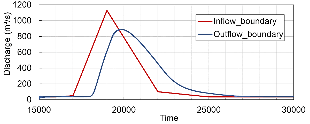
Figure 2:Die simulierten Flüsse fließen über die stromaufwärtigen Inflow boundary und die stromabwärtigen Outflow boundary Steuerabschnitte.
Der Peak-Zufluss entspricht den angegebenen 1130 m/s, während der Outflow-Peak-Abfluss nur 889 m/s beträgt und der Peak etwa 1070 Sekunden dauert (Einfluss bei =19000 und Abfluss bei 20070), um durch den Abschnitt zu gelangen.
Resolve volume balance issues in unsteady simulations
Die gesamten Zu- und Abflussvolumina in der hier vorgestellten Simulation betragen 3479930,958 m bzw. 3430100,437 m. Es gibt also einen Gesamtvolumenfehler von 1,4. Um solche Probleme zu überwinden, empfiehlt das Telemac2d-Handbuch], einen Mindestwert für die Wassertiefe zu verwenden, um zu definieren, wann eine Zelle nass oder trocken ist. Gleichzeitig empfehlen die Entwickler für die meisten Simulationen keine Mindestwassertiefe und betonen, diese Option nur für instationäre (quasi-stationäre) Simulationen zu verwenden. Um eine minimale Wassertiefe zu definieren, muss das Schlüsselwort BEHANDLUNG DER TIDALFLATEN auf 2 gesetzt werden (lesen Sie mehr unter steady2d tutorial), was weder mit Parallelisierungsroutinen noch mit den hier verwendeten SCHEME FOR ADVECTION ... : 14-Einstellungen kompatibel ist. Bessere Ergebnisse, aber lange nicht-parallelisierte quasi-stationäre Berechnungen könnten mit den folgenden Schlüsselwörtern in der Steuerungsdatei erzielt werden:
OPTION FOR THE TREATMENT OF TIDAL FLATS : 2 / use segment-wise flux control
MINIMUM VALUE OF DEPTH : 0.1 / in meters
Visualisierung mit QGIS
The results of the unsteady simulation can be visualized and snapshots exported to raster (e.g., GeoTIFF) or shapefile formats in QGIS, similar as explained in the steady2d post-processing. Specifically, the latest QGIS releases enable to load the Selafin results mesh file (here: r2dunsteady.slf) as a QGIS mesh layer. Therefore, launch QGIS, go to the Layer menu and click on Add Layer > Add Mesh Layer.... In the popup window (Data Source Manager / Mesh), select r2dunsteady.slf, click Add, and Close. Figure 3 shows the imported r2dunsteady mesh layer in QGIS with a Softlight blending (set in the Symbology) on google satellite imagery.
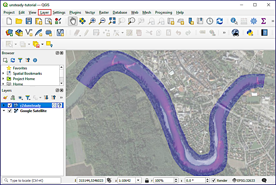
Figure 3:Die instationäre (quasi-steady) Simulationsergebnisse-Datei r2dunsteady.slf importiert als Mesh-Layer in QGIS und überlagert auf Google Satellitenbilder Google, n.d..
r2dunsteady.slf (results file) not correctly showing in QGIS
Wird die Ergebnisdatei r2dunsteady.slf nicht in QGIS angezeigt? Importieren Sie es mit der korrekten Georeferenz: EPSG:32633 (ETRS 89 / UTM Zone 33N).
The simulation output parameters (e.g., U, V, or Q) at a selected timestep can be controlled in the layer properties of the r2dunsteady layer (double-click on it in the Layers panel).
To create a video of simulation results, use the Time Controller (see activation in Fig. 4). The frequency of images can be set through clicking on the cogwheel of the time controller, and image sequences played by clicking in the Play button. Additionally, Fig. 5 uses an overlay of water depth pixel colors (contour plot), and flow velocity vectors, defined in the Layer Styling panel. The North and discharge arrows, and the title are Decorators, which can be found in View > Decorators.
Die exportierte Bildserie kann mit Videobearbeitungssoftware in ein Video konvertiert werden, z. B. die einfach und kostenlos zu verwendenden OpenShot (gut für Windows) oder kdenlive (gut für Linux) Werkzeuge. Die unten gezeigte Box enthält ein beispielhaftes Video, das mit kdenlive] erstellt wurde.
Expand to view the results as video
Sebastian Schwindt @ Hydro-Morphodynamics channel on YouTube.
- Gifford-Miears, C., & Leon, A. (2013). Tutorial on the use of TELEMAC-2D Hydrodynamics model and Pre-/Post-processing with BlueKenue for flood-inundation mapping in Unsteady Flow Conditions. Oregon State University. https://web.eng.fiu.edu/arleon/courses/Transient_flows/Tutorials/TELEMAC_2D/TELEMAC_2D_Tutorial_Baxter.pdf
- Google. (nd). Google Satellite Imagery. https://mt1.google.com/vt/lyrs=s&x=%7Bx%7D&y=%7By%7D&z=%7Bz%7D