Reibungszonen
Similar to the assignment of multiple friction coefficient values to multiple model regions featured in the BASEMENT tutorial, Telemac2d provides routines for domain-wise (i.e., zonal) friction area definitions in the geometry (.slf) mesh file. Specifically, if the study domain is characterized by regions of different roughness, it is not sufficient to define global friction through a FRICTION COEFFICIENT keyword in the steering (.cas) file. Defining roughness zones in the mesh (.slf) file requires an additional layer called BOTTOM FRICTION or FRIC_ID on top of the BOTTOM elevation. To this end, roughness values can be defined in a roughness .xyz file created with QGIS (recommended) or Closed Lines .i2s created with BlueKenue (see the meshing section). While QGIS is recommended to delineate roughness zones with correct and possibly precise georeferences, BlueKenue is still required for interpolating the roughness from the .xyz or .i2s file on the .slf file in the last step.
Roughness.XYZ mit QGIS (empfohlen)
Der erste Schritt zur Abgrenzung von Rauheitszonen in QGIS besteht darin, das Koordinatenreferenzsystem einzurichten und das Projekt analog zum QGIS pre-processing tutorial zu speichern:
Öffnen Sie QGIS und gehen Sie im oberen Menü zu Project > Properties.
Aktivieren Sie den Koordinatenreferenzsystem-Tab.
Set the CRS that your basemap / Digitales Oberflächenmodell data use; for this example, enter
UTM zone 33Nand select UTM zone 33N (WGS84) (EPSG 32633), which is not a great choice because of its low precision, but it will do the job for this tutorial.Klicken Sie auf Apply und OK.
Speichern Sie das Projekt in einem neuen Ordner, in dem alle Dateien für dieses Tutorial gespeichert werden.
Es wird wichtig sein, Überschneidungen zu vermeiden, die zu mehrdeutigen oder fehlenden Definitionen von Regionen führen würden. Aktivieren Sie daher Snapping:
Aktivieren Sie die *Snapping Toolbar *: **View * > **Snapping Toolbar *
In der Snapping-Symbolleiste > Snapping aktivieren

Ermöglichen Sie Snaping für
Vertex, Segment und Mitte der Segmente
 .
.Snapping on Intersections
 .
.Self Snapping
 .
.
This tutorial picks up the example from the Telemac QGIS pre-processing tutorial to draw polygons along the breaklines and liquid-boundaries shapefiles. The friction zones are inferred from a Google Satellite basemap and friction attributes are qualitatively estimated, which is just fine for a tutorial. In practice, we strongly recommend performing field surveys on grain size distributions with high-precision differential GPS (DGPS) systems to delineate roughness zones on-site supported by drone imagery.
Abgrenzung von Rauhigkeitszonenpolygonen
Die Rauhigkeitszonen können durch Attribute eines Polygon-Shapefiles beschrieben werden. Um eine neue Polygon-Shapefile zu erstellen, gehen Sie zu Layer > Create Layer > New Shapefile Layer... (siehe Fig. 1).
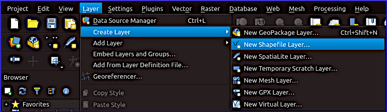
Figure 1:Erstellen Sie ein neues Polygon Shapefile.
Geben Sie im Popup-Fenster die folgenden Definitionen ein:
Dateiname: Drücken Sie ..., navigieren Sie zum Projektordner und tippen Sie auf
friction-polygons.Dateicodierung: Standard beibehalten (Probedateien verwenden
UTF-8).Geometrietyp:
PolygonUnterhalb der *Zusätzlichen Dimensionen * (nicht erforderlich) finden und klicken Sie auf die Schaltfläche **Koordinatenreferenzsystem **, um das oben definierte Projektkoordinatensystem auszuwählen (Beispieldateien:
EPSG:32633).Fügen Sie ein neues Feld hinzu:
Name:
dMeanTyp:
Decimal (double)Länge:
10Präzision:
5Klicken Sie auf Add to Fields List
Fügen Sie ein weiteres Neues Feld hinzu:
Name:
fricIDTyp:
Integer (32 bit)Länge:
5Klicken Sie auf Add to Fields List
Drücken Sie OK, um das neue Shapefile zu erstellen.
To follow this tutorial, import the breaklines (download as zip-file) and liquid-boundaries (download as zip-file) shapefiles from the Telemac pre-processing. To draw polygons by editing fiction-polygons.shp along the breaklines and liquid boundaries, highlight fiction-polygons in the Layers panel, and enable editing by clicking on the yellow pen  . Activating Add Polygon Feature and draw polygons by snapping to points of the breaklines and liquid boundaries layers, according to Fig. 2. To finalize each polygon with a right-click on the mouse and enter the
 fricID and dMean values according to Tab. 1 (qualitative grain sizes).
To correct drawing errors use the Vertex Tool  . Finally, save the new polygons (edits of friction-zones.shp) by clicking on the Save Layer Edits
  symbol. Stop (Toggle) Editing by clicking again on the yellow pen symbol.
Alternatively, merge the breaklines and liquid boundaries, and use the Polygonize tool from the Processing Toolbox to convert the merged lines into a polygon shapefile. However, the polygonization will miss some breaklines, which will require editing. Also, the fricID and dMean fields still need to be added through editing.
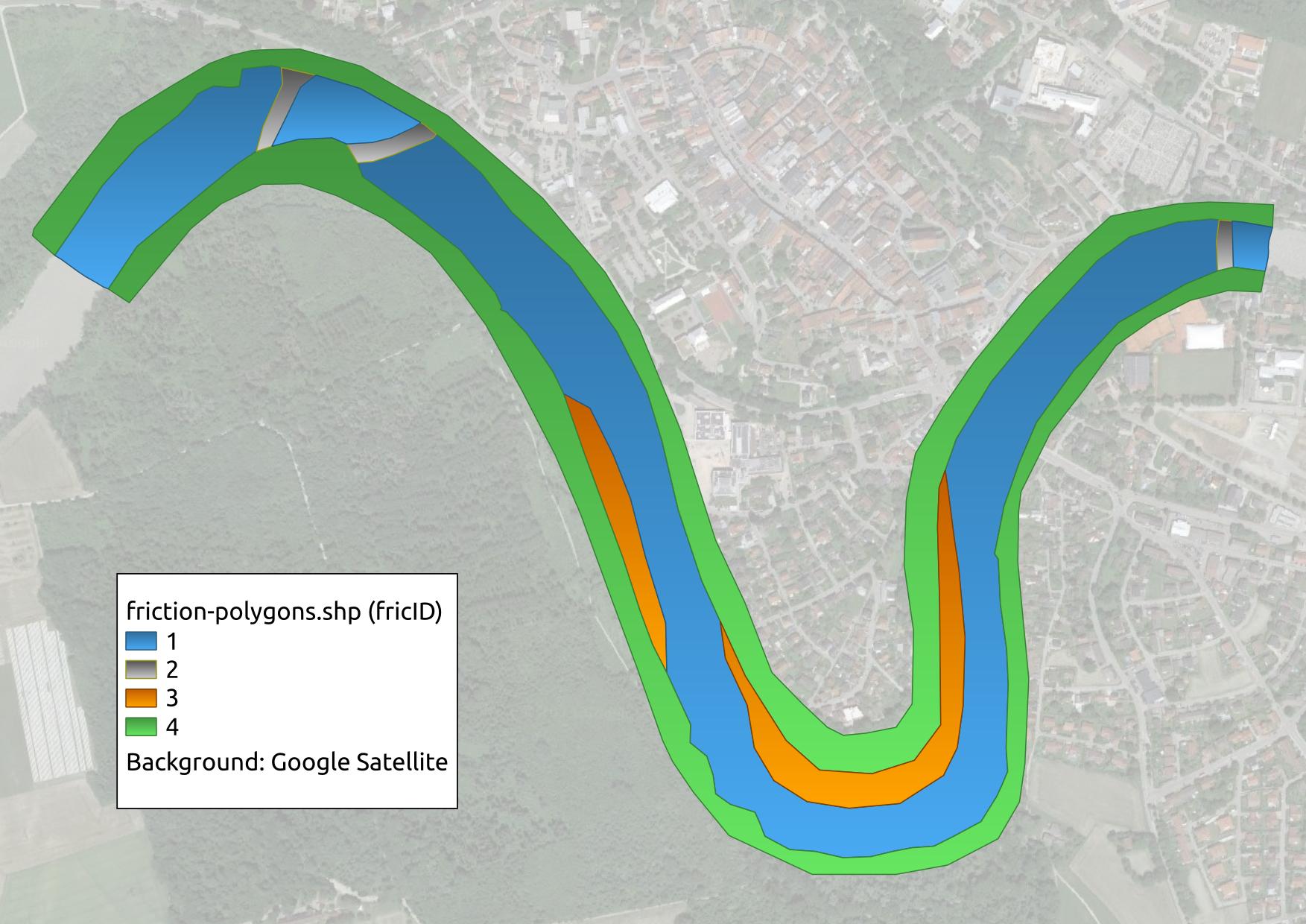
Figure 2:Beispiel für die Beschreibung von Rauheitszonen (Reibungszonen) mit Polygonen durch vier Reibungs-IDs (fricID), die (1) das Flussbett, (2) Blockrampen, (3) Schotterstäbe und (4) Auen begrenzen. Hintergrundkarte: Google (n.d.) Satellitenbilder.
Table 1:Four exemplary friction zones described by integer fricIDs and mean grain size diameters dMean.
Zonenbezeichnung | Flussbett | Blockrampen | Grasbanken | Überschwemmungsgebiete |
|---|---|---|---|---|
Fricid | 1 | 2 | 3 | 4 |
dMittelwert (m) | 0,080 | 0,300 | 0,033 | 1.000 |
Rauhigkeitspunkte erzeugen
Der nächste Schritt auf dem Weg zum Erstellen der erforderlichen XYZ-Datei zum Zuweisen von Reibungszonen zu einer Selafin-Geometrie-Datei besteht darin, (zufällige) Punkte innerhalb der oben erstellten Polygone zu erzeugen. Zu diesem Zweck geben Sie random points inside polygons** im Feld search der Processing Toolbox ein. Im Popup-Fenster Random Points Inside Polygons (Fig. 3) geben Sie Folgendes ein:
Eingabeschicht:
friction-polygonsSampling-Strategie:
Points densityPoint count or density:
0.25- use a smaller/larger value for fine/coarse meshes, but beware of potentially very large file sizesMinimum distance between points:
5.0- use a smaller/larger value for fine/coarse meshesRandom points: click on ... and define a target point shapefile name, such as
friction-pts.shpto be stored in the project folder.Klicken Sie auf Run, um die Punkte Shapefile zu erstellen. Dieser Vorgang kann je nach definierter Punktdichte eine Weile dauern.
The resulting point shapefile is shown in Fig. 4.
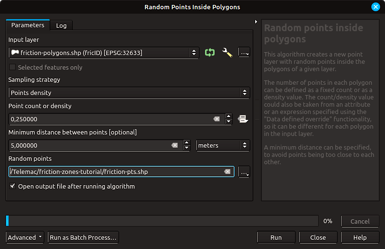
Figure 3:Einstellungen im Tool Random Points Inside Polygons in QGIS. Wählen Sie sorgfältig die Punktzahl oder Dichte aus, was sehr große Ausgabedateien verursachen kann. Das Mindestabstandsfeld kann verwendet werden, um die Anzahl der Punkte zu reduzieren.
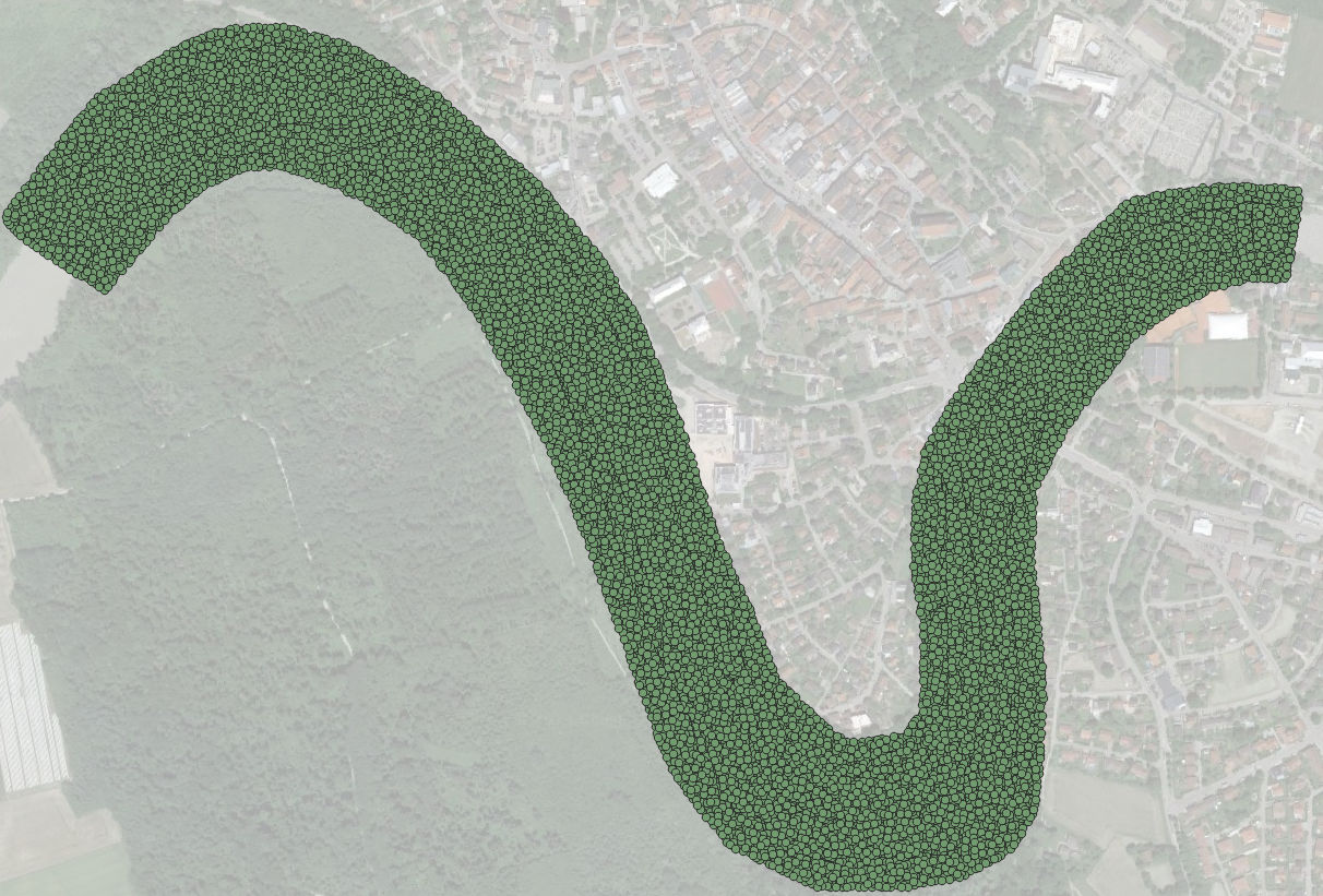
Figure 4:Die Punktformdatei, die sich aus der Verwendung des Tools Random Points Inside Polygons in QGIS ergibt. Hintergrundkarte: Google (n.d.) Satellitenbilder.
Zuweisen von Reibungsattributen zu Punkten
Leider nimmt die Punktgenerierung die Polygonattribute nicht automatisch auf, die auf die Punkte interpoliert werden müssen. Abhängig vom angestrebten Rauheitsgesetz für die Verwendung mit Telemac können entweder die Reibungs-IDs oder direkt Rauheitskoeffizienten zur Attributtabelle des Friktionspunkt-Shapefiles hinzugefügt werden. In diesem Tutorial wird ein Reibungskoeffizient in Form der Strickler-Rauheit interpoliert und mit einer empirischen Formel berechnet. Ein komplexerer Fall für die Berechnung von Rauheitswerten findet sich in der Fallstudie Donau (Donau) der BAW (unter HOMETEL/examples/telemac2d/donau/).
Die Übertragung der dMean und/oder fricID-Attribute der Polygone zu den Punkten ist im Wesentlichen eine Interpolationsoperation, bei der QGIS jeden Punkt betrachtet und ihm die dMean und/oder fricID-Attribute des nächstliegenden Polygons zuweist. Klicken Sie dazu auf das Vector Top-Menü > Data Management Tools > Join Attributes by Location (siehe Fig. 5).
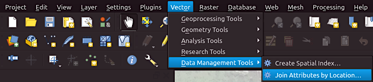
Figure 5:Öffnen Sie das Join Attributes by Location Tool in QGIS.
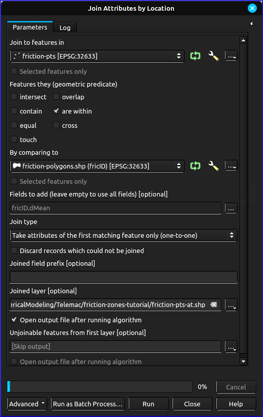
Figure 6:Öffnen Sie die Attributtabelle der Friktionspunkttabelle.
Führen Sie im Popup-Fenster (Fig. 6) die folgenden Einstellungen durch:
** Verbinden Sie sich mit Features in**:
friction-ptsFeatures they (geometric predicate): check the
are withinbox, deselect all othersDurch Vergleich mit:
friction-polygons** Zum Hinzufügen von Feldern**: Klicken Sie auf die Schaltfläche ..., um
fricIDund/oderdMeanJoin type:
Take attributes of the first matching feature only (one-to-one)Joined layer: Klicken Sie auf die Schaltfläche ... > Speichern zur Datei > Navigieren Sie zum ** Projektordner** > ** Geben Sie einen Dateinamen ein, z. B.
friction-pts-at**Klicken Sie auf Run.
Die Fehlermeldung *Kein räumlicher Index existiert für die Eingabeschicht, die Leistung wird stark beeinträchtigt * kann für diese Anwendung ignoriert werden. Um jedoch eine falsche Ausgabe zu überprüfen, ist es möglicherweise ratsam, auch die Schicht **Unverbindliche Merkmale der ersten Schicht ** zu definieren.
Infolgedessen ist das friction-pts-at im Layers-Panel verfügbar (siehe Fig. 7).
Um die mittleren Korngrößen (dMean) in Reibungswerte umzuwandeln, öffnen Sie die Attributtabelle durch ** Rechtsklick** auf der ** Reibung-pts-at**-Schicht im Layers-Panel > Offene Attributtabelle.
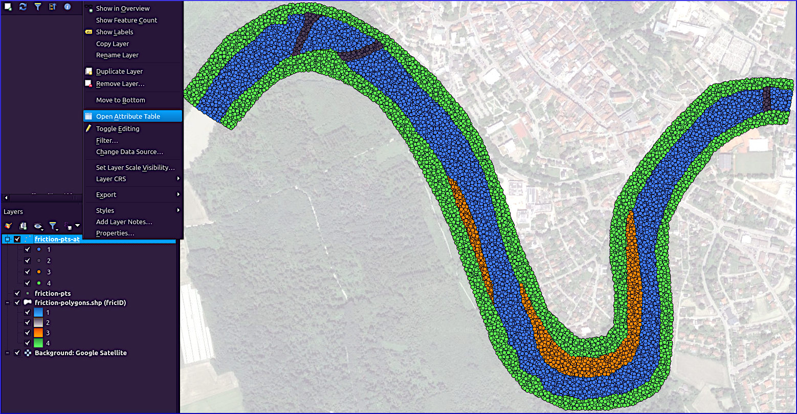
Figure 7:Öffnen Sie die Attributtabelle der Friktionspunkt-Shapefile mit Attributtabelle. Hintergrundkarte: Google (n.d.) Satellitenbilder.
Bearbeiten Sie die Attributtabelle (Fig. 8):
Editing ermöglichen,
remove unnecessary columns, such as the
idfield, and potentially also thefricIDfield (this showcase will only use thedMeancolumn),Öffnen Sie den **Feldrechner **, mit dem wir im nächsten Schritt Strickler-Rauheitswerte ableiten werden.
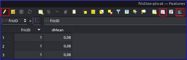
Figure 8:Die Attributtabelle der Friction-pts-at-Schicht mit den hervorgehobenen (roten Rechtecken) Bearbeiten, Entfernen von Spalten und Feldrechnertasten (von links nach rechts).
Optional: derive x and y coordinates with the Field Calculator
Fügen Sie im Feldrechner die Koordinaten und zur Attributtabelle hinzu:
Kontrollieren Sie das Kontrollkästchen Ein neues Feld erstellen
Ausgabefeldname:
x_coordAusgabefeldtyp:
Decimal number (real)Ausgabefeldlänge:
10und Präzision:10Geben Sie eine Formel ein, indem Sie entweder den x-Wert aus der Geometrie in der Scrollbox auswählen oder direkt in das Feld Expression eingeben:
x( @geometry ) In analoger Weise fügen Sie y_coord mit hinzu:
y( @geometry ) ** Speichern Sie die Bearbeitungen in der Attributtabelle, indem Sie auf das Festplattensymbol klicken.
According to Meyer-Peter & Müller (1948), the Strickler (1923) roughness (friction) coefficient can be approximated with 26/ based on the grain size , where 90% of the surface sediment grains are smaller. In addition, we will assume that Rickenmann & Recking, 2011. Thus, . To run this calculation, go to the Field Calculator and (see Fig. 7):
Kontrollieren Sie das Kontrollkästchen Ein neues Feld erstellen
Ausgabefeldname:
k_stAusgabefeldtyp:
Decimal number (real)Ausgabefeldlänge:
3und Präzision:2Geben Sie eine Formel ein, indem Sie entweder
dMeanausFields and Valuesin der Scrollbox auswählen oder direkt die Gleichung in das Feld Expression eingeben:
26 / ( ( 2.25 * "dMean" ) ^ ( 1 / 6 ) )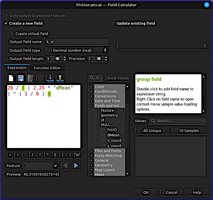
Figure 9:Schätzen Sie den Strickler-Koeffizienten basierend auf der mittleren Korngröße (dMean) mit dem Feldrechner in QGIS.
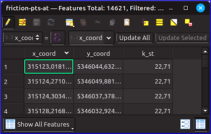
Figure 10:Die finalisierte Attributtabelle der Friktion-pts-at-Schicht mit den optionalen x- und y-Koordinaten und den geschätzten Strickler-Rauheitskoeffizienten.
Schließlich entfernen Sie alle verbleibenden unnötigen Felder** aus der Attributtabelle und speichern Sie die Bearbeitungen, indem Sie auf das Festplattensymbol klicken und die Bearbeitung umschalten (d. H. Deaktivieren).
Exportpunkte nach XYZ
Beginnen Sie mit dem Öffnen des Export-Dialogs mit einem Rechtsklick auf die Friktion-pts-at-Schicht > Export > Funktionen speichern als ... (Fig. 11).
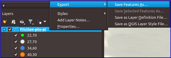
Figure 11:Öffnen Sie den Exportdialog mit einem Rechtsklick auf die Friction-pts-at-Schicht > Export > Features speichern als...
Führen Sie im Vector Layer als... Popup-Fenster die folgenden Einstellungen aus (Fig. 12):
Format:
Comma Separated Value [CSVDateiname: Klicken Sie auf ..., navigieren Sie zum Projektordner und geben Sie
friction-pts.xyzfür den Dateinamen ein (drücken Sie Speichern).Layername: klar halten
Koordinatenreferenzsystem: Stellen Sie sicher, dass das Koordinatenreferenzsystem der Friction-pts-at-Schicht definiert ist (im Showcase
EPSG:32633 - WGS 84 / UTM zone 33N)Encoding: standardmäßig verwenden (im Showcase
UTF-8)**Wählen Sie alle relevanten **Felder ** aus, das heißt im Showcase mindestens
k_st. Die optionalen Felderx_coordundy_coordsind nur erforderlich, wenn die Geometrie nicht exportiert wird (aus welchem Grund auch immer).**Überprüfen Sie die **Persist-Schicht Metadaten **
Geometrietyp:
Automatic(meist standardmäßig)Scrollen Sie nach unten zu den Layer-Optionen und:
Setzen Sie das GEOMETRY auf
AS_XYSetzen Sie den SEPARATOR auf
TAB
** Deaktivieren Sie die **Gespeicherte Datei hinzufügen, um das Feld ** unten im Fenster abzubilden.
** Halten Sie alle anderen Standardeinstellungen** und klicken Sie auf OK.
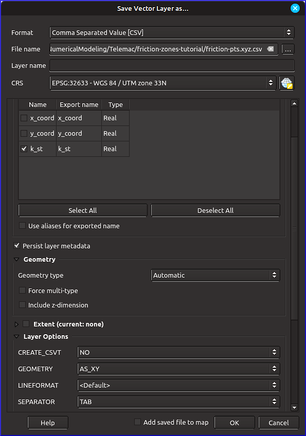
Figure 12:Einstellungen im Speichern von Vektorschicht als... Popup-Fenster zum Exportieren der Friktionspunkte in eine XYZ-Datei (tab-separated CSV).
QGIS will have exported the file with a .xyz.csv ending. Rename the file to remove .csv at the end. Verify the correct formatting of the .xyz file by opening it in a text editor (e.g., Notepad++). For instance, if you calculated and exported the x_coord and y_coord fields, and additionally the geometry, the .xyz file will hold two times the coordinates. In this case, import the .xyz file in a spreadsheet editor (i.e., office application), delete the x_coord and y_coord columns, and re-export the file as a tab-separated CSV file. Read more about .xyz file conversion in the QGIS tutorial.
Expand to see the correct header of the showcase friction-pts.xyz file
X Y k_st
315976.648906296  5345616.71281044  40.30
315992.808134594  5345521.13037269  40.30
315983.283370604  5345655.68430873  40.30
315915.433790676  5345754.82689794  40.30
[...]Alternative: Friktionszonen in BlueKenue zeichnen
Dieses Verfahren ist eine ungenaue Alternative zu der oben beschriebenen roughness.xyz-Erstellung aufgrund der schwachen geospatialen Referenzierungskapazitäten von BlueKenue, weshalb das unten stehende instruction box nur zur Vollständigkeit vorgesehen ist.
Unfold to read this non-recommended alternative
Beginnen Sie mit dem Erstellen neuer geschlossener Linien (Fig. 13), ähnlich wie Polygone, die Rauheitszonen abgrenzen.
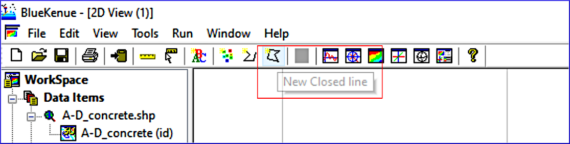
Figure 13:Einstellungen im Speichern von Vektorschicht als... Popup-Fenster zum Exportieren der Friktionspunkte in eine XYZ-Datei (tab-separated CSV).
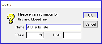
Figure 14:Weisen Sie dem durch die geschlossene Linie abgegrenzten Bereich einen Reibwert (Rauheit) zu (hier: eine Strickler-Rauheit von 50).
After drawing a Closed line is finished, press the Esc key and the window shown in Fig. 14 will appear, where a roughness value can be assigned. The exemplary figure assigns a Strickler roughness of 50 in the Value field to a Closed line named A-D_substrate. Continue to assign names to all relevant roughness areas.
Finally, save the Closed line objects as .i2s / .i3s files.
Zonal Friction Mesh (BlueKenue)
In diesem Abschnitt wird die Interpolation von Reibungswerten in einer vorhandenen Geometriedatei mit Selafin (.slf) durchlaufen. Das Schaufenster baut auf der .slf-Datei auf, die im Telemac pre-processing tutorial erstellt wurde (download qgismesh.slf). Beginnen Sie mit ** Öffnen von BlueKenue ** und öffnen Sie die Datei selafin .slf: Klicken Sie auf **File ** > Open... > Navigieren Sie zu dem Verzeichnis, in dem der .slf gespeichert ist, wählen Sie **Telemac Selafin File (*.slf) ** aus, markieren Sie qgismesh.slf und drücken Sie **Open **. Ziehen Sie die Ebene BOTTOM (BOTTOM) aus den Workspace-Datenelementen in Views > 2D View (1), um den korrekten Import des Meshs zu überprüfen und zu visualisieren (Fig. 15).
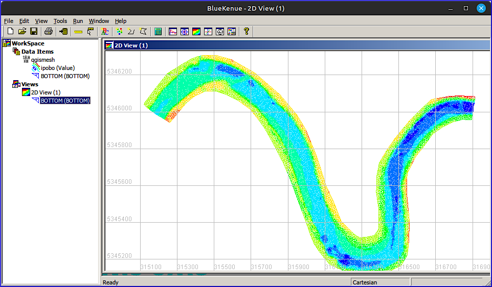
Figure 15:Die Datei qgismesh.slf selafin wurde in BlueKenue geöffnet.
Einfuhrfriktionszonen
Als Alternative zur Erstellung von zonalen Reibungswerten, die in einer mit QGIS generierten .xyz-Datei gespeichert sind, können Zonen auch direkt in BlueKenue durch eine Reihe von * Geschlossenen Linien * gezeichnet werden. Aufgrund der sehr begrenzten Kapazitäten von BlueKenue, um mit geospatialen Referenzen und Koordinatensystemen (CRSs) umzugehen, ist **die bevorzugte Option ** zum Erstellen von Reibungszoneneingaben ** die oben beschriebene Anwendung von **QGIS **.
To open the above-created .xyz file in BlueKenue:
Klicken Sie auf File > Open...
Navigieren Sie zum Projektordner, in dem
.xyzgespeichert istWählen Sie Alle Dateien (*.*) neben dem Feld Dateiname: aus.
highlight
qgismesh.slf, and press Open.
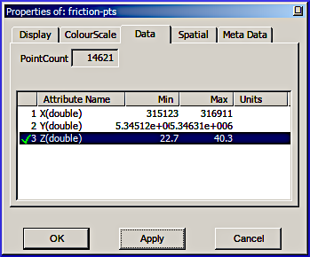
Figure 16:Weisen Sie dem durch die geschlossene Linie abgegrenzten Bereich einen Reibwert (Rauheit) zu (hier: eine Strickler-Rauheit von 50).
Ignoriere die Warnung Nachricht (klicke OK). Um die importierten Reibungswerte zu überprüfen und zu visualisieren Rechtsklick auf der ** Friction-pts (X)** Schicht > Eigenschaften > gehen Sie auf die Registerkarte Daten > ** Wählen Sie Z(double)**, drücken Sie Apply. Gehen Sie dann zur Registerkarte ColourScale, drücken Sie Reset, Apply und OK.
Überprüfen Sie die korrekte Darstellung der Reibungswerte, indem Sie die friction-pts (Z)-Schicht aus den Workspace-Datenelementen in Views > 2D View (1) (Fig. 17) ziehen.
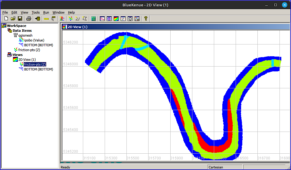
Figure 17:Die importierte Friction-pts.xyz-Datei (erstellt mit QGIS) visualisiert in BlueKenue.
If not yet done, import the Closed lines delineating roughness zones in the form of .i2s / .i3s files.
Interpolationsreibung am Mesh
Gehen Sie in BlueKenue zu File > New > 2D Interpolator, der im Work Space > Data Items auftritt. Drag & drop entweder die friction-pts .xyz-Punkte oder die Closed line-Objekte, die Rauheitszonen abgrenzen auf dem neuen 2D Interpolator (siehe Fig. 18).
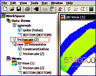
Figure 18:Ziehen Sie die Reibungspunkte (oder geschlossenen Linien) auf einem neuen 2D-Interpolator in BlueKenue.
Als nächstes fügen Sie eine neue Variable zum qgismesh.slf-Mesh hinzu, indem Sie das Selafin qgismesh-Objekt hervorheben (in Work Space > Data Items) und Rechtsklick darauf. Klicken Sie auf Variable hinzufügen... und geben Sie im Popup-Fenster Folgendes ein (Fig. 19 oder Fig. 20), je nachdem, ob Sie mit Reibungswerten arbeiten (wie hier mit Strickler-Rauheit dargestellt), oder friction IDs (see below):
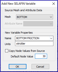
Figure 19:Fügen Sie dem Selafin-Objekt eine neue Variable für direkte Reibungswerte hinzu.
Mesh:
BOTTOM**Name:
BOTTOM FRICTION(dieses Beispiel)Einheiten: Freihalten (irrelevantes Feld)
Standard-Knotenwert:
30(in diesem Beispiel) für einen Standardwert (Strickler), der verwendet werden kann, wenn keine xyz-Reibungspunkte in der Nähe eines Mesh-Knotens gefunden werden können
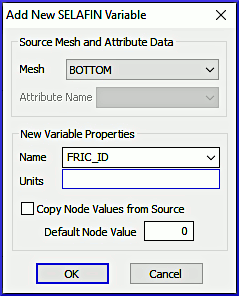
Figure 20:Fügen Sie eine neue Variable zum Selafin-Objekt für Reibungs-IDs hinzu.
Mesh:
BOTTOMName:
FRIC_ID(muss eingegeben werden, kann nicht aus der Liste ausgewählt werden)Einheiten: Freihalten (irrelevantes Feld)
Standard Node Value:
0(ID zu verwenden, wenn keine xyz-Punkte in der Nähe eines Mesh-Knotens gefunden werden können)
To interpolate the friction values on the mesh, highlight the new variable variable BOTTOM FRICTION (or FRIC_ID) of the qgismesh object in Work Space > Data Items. The Anonymous Attribute of the new variable can be ignored. To map the new variable onto the mesh:
Hervorheben der neuen
BOTTOM FRICTION(oderFRIC_ID) Mesh-Variablen (in Datenelemente)Gehen Sie zu Tools > Map Object... (Top-Menü unter Fig. 21)
Wählen Sie den neuen 2D-Interpolator und klicken Sie auf OK, wodurch das Popup-Fenster Processing... geöffnet wird.
Nachdem die Verarbeitung abgeschlossen ist, klicken Sie auf OK.
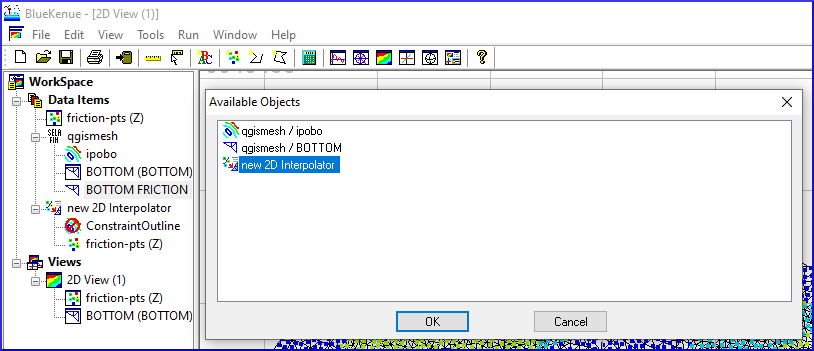
Figure 21:Karte den Reibungswert auf dem neuen 2D Interpolator in BlueKenue.
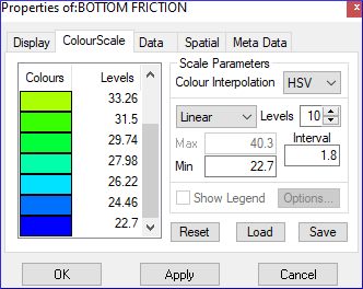
Figure 22:Passen Sie die Farbskala für Bottom Frederick an.
Überprüfen Sie die korrekte Interpolation:
Definieren Sie eine relevante Farbskala:
In Work Space > Data Items > qgismesh, right-click auf die neue BOTTOM FRICTION Variable > Eigenschaften.
In the properties, go to the ColourScale tab, and use, for example, a Linear scale with
10Levels, a Min of22, and an Interval of1.8. The exemplary minima and interval are good choices for the showcase, but other settings might be preferable for other applications (e.g., prefer Min of0when using Manning’s ).Drücken Sie Apply > OK.
Drag & drop die Variable BOTTOM FRICTION in Views > 2D View (1), um die korrekte Interpolation der Reibungswerte zu überprüfen (z.B. siehe Fig. 23 für das Schaufenster).
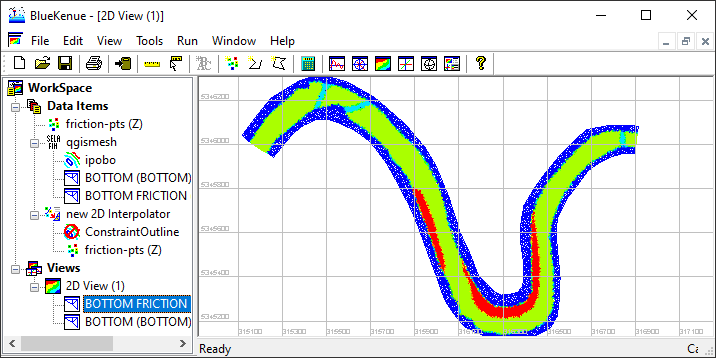
Figure 23:Die korrekt interpolierte neue BOTTOM FRICTION-Variable des qgismesh.slf-Meshs.
Um den Selafin **mesh ** mit interpolierten interpolierten Reibungswerten zu speichern ** Rechtsklick ** auf das qgismesh-Selafin-Objekt ** > Eigenschaften > gehen Sie auf die Registerkarte Meta-Daten und geben Sie einen neuen Name ein, z. B. qgismesh-friction. Als nächstes markieren Sie das Selafin-Objekt (z.B. qgismesh-friction) und klicken Sie auf das Symbol  . Wenn die Umbenennung für den Dateinamen nicht wirksam wurde, bestätigen Sie das Ersetzen der vorhandenen Datei.
Telemac-Bindungen
Umsetzung in der CAS-Datei
Friction Keywords
The updated qgismesh-friction.slf mesh can be used just like in the steady 2d tutorial, but some keywords need to be modified, even though the BOTTOM FRICTION values assigned in the .slf mesh automatically overwrite the global FRICTION COEFFICIENT keyword in the .cas steering file. However, we need to make Telemac recognize the newly defined BOTTOM FRICTION zones as Strickler roughness type. To this end, change the LAW OF BOTTOM FRICTION to 3 (instead of 4 pointing to Manning’s ), and set the default FRICTION COEFFICIENT to 33 (inverse of = 0.03). The definition of the FRICTION COEFFICIENT is for coherence and is not strictly needed as it will be overwritten by the BOTTOM FRICTION from the .slf mesh.
/ steady2d-zonal-ks.cas steering file
/ ...
/ Friction at the bed
LAW OF BOTTOM FRICTION : 3 / 3-Strickler
FRICTION COEFFICIENT : 33  / will be overwritten by zonal friction values
/ steady2d.cas steering file
/ ...
/ Friction at the bed
LAW OF BOTTOM FRICTION : 4 / 4-Manning
FRICTION COEFFICIENT : 0.03 / Roughness coefficientAdd the letter W to the graphic printouts for writing the friction coefficient to the results file:
/ steady2d-zonal-ks.cas steering file
/ ...
VARIABLES FOR GRAPHIC PRINTOUTS : 'U,V,H,S,Q,W' / add W for friction coefficient
Do you have more than 10 different friction zones?
Um die Anzahl der von Telemac erkannten Reibungszonen zu erhöhen, setzen Sie das Schlüsselwort MAXIMUM NUMBER OF FRICTION DOMAINS, zum Beispiel auf 20:
/ steady2d-zonal-ks.cas steering file
/ ...
MAXIMUM NUMBER OF FRICTION DOMAINS : 20 / default is 10
Startbedingungen (fakultativ)
Die folgenden Beschreibungen beziehen sich auf Abschnitt 4.1.3 im Telemac2d Manual.]
To speed up the simulation, this tutorial re-uses the output of the steady 2d simulation (though, re-created with a printout period of 2500 steps). This type of model initialization is also called hotstart, here, based on the steady results file r2dsteady-t15k.slf, which needs to be defined as PREVIOUS COMPUTATION FILE:
/ steady2d-zonal-ks.cas steering file
/ ...
COMPUTATION CONTINUED : YES
PREVIOUS COMPUTATION FILE : r2dsteady-t15k.slf / results of 35 CMS steady simulation after 15000 timesteps
Mit den Hotstart-Bedingungen können die Grenzen erleichtert werden:
/ steady2d-zonal-ks.cas steering file
/ ...
/ Liquid boundaries
PRESCRIBED FLOWRATES  : 35.; 0.
PRESCRIBED ELEVATIONS : 0.; 371.33
Damit diese Randbedingungen wirksam werden können, muss die Datei mit flüssigen Grenzen aus der stetigen 2D-Simulation geändert werden:
open boundaries.cli in einem text editor
find the
5 5 5(prescribed Q and H) upstream boundary and replace it with4 5 5(prescribed Q only)speichern und schließen boundaries.cli
for more information, have a look at the spotlight chapter on boundary conditions
alternativ download der angepassten borders.cli here].
Finally, comment out any initial conditions keywords in the .cas steering file, for instance:
/ steady2d-zonal-ks.cas steering file
/ ...
/ INITIAL CONDITIONS : 'ZERO DEPTH'
/ INITIAL DEPTH : 0.005
Run Friction Zone Simulation
Make sure all required files are placed in a simulation folder (e.g., /HOME/modeling/friction-tutorial/), notably:
die qgismesh
-friction .slf mesh mit BOTTOMundBOTTOM FRICTIONInformationen]korrigiert boundaries.cli]
die r2dsteady-t15k.slf Results-Datei, um den Hotstart zu aktivieren]
die steady2d
-zonal -ks .cas Steering-Datei mit aktualisierten Schlüsselwörtern].
Navigate (cd) to the Telemac installation directory (HOMETEL) to activate (source) the Telemac environment in Terminal (use the same environment as for compiling Telemac):
cd ~/telemac/v9.0.0/configs
source pysource.gfortranHPC.sh
Als nächstes cd in den Simulationsordner und führen Sie die Simulation, möglicherweise mit dem -s Flag, um flux convergence zurückzuverfolgen:
cd ~/modeling/friction-tutorial/
telemac2d.py steady2d-zonal-ks.cas -s
Der erfolgreiche Simulationslauf wird mit so etwas beendet sein:
Unfold to see the expected Terminal output
================================================================================
 ITERATION    10000    TIME:  6 H 56 MIN  40.0000 S   (    25000.0000 S)
--------------------------------------------------------------------------------

[...]

--------------------------------------------------------------------------------
                       BALANCE OF WATER VOLUME
     VOLUME IN THE DOMAIN :    268926.5     M3
     FLUX BOUNDARY    1:     35.00000     M3/S  ( >0 : ENTERING  <0 : EXITING )
     FLUX BOUNDARY    2:    -34.99963     M3/S  ( >0 : ENTERING  <0 : EXITING )
     RELATIVE ERROR IN VOLUME AT T =       0.2500E+05 S :    0.2327571E-14
--------------------------------------------------------------------------------
                   FINAL BALANCE OF WATER VOLUME

     RELATIVE ERROR CUMULATED ON VOLUME:    0.4112446E-14

     INITIAL VOLUME              :     268899.0     M3
     FINAL VOLUME                :     268926.5     M3
     VOLUME THAT ENTERED THE DOMAIN:     27.48362     M3  ( IF <0 EXIT )
     TOTAL VOLUME LOST             :    0.1105946E-08 M3

 END OF TIME LOOP

 EXITING MPI

                     *************************************
                     *    END OF MEMORY ORGANIZATION:    *
                     *************************************

 CORRECT END OF RUN

 ELAPSE TIME :
                              3  MINUTES
                              3  SECONDS
Note: The following floating-point exceptions are signalling: IEEE_UNDERFLOW_FLAG IEEE_DENORMAL
STOP 0

... merging separated result files

... handling result files

        moving: r2dsteady-ks-zonal.slf
      copying: steady2d-zonal-ks.cas_2030-07-28-14h55min04s.sortie
... deleting working dir


My work is done
Die resultierenden flux convergence und convergence rates sollten ähnlich aussehen:
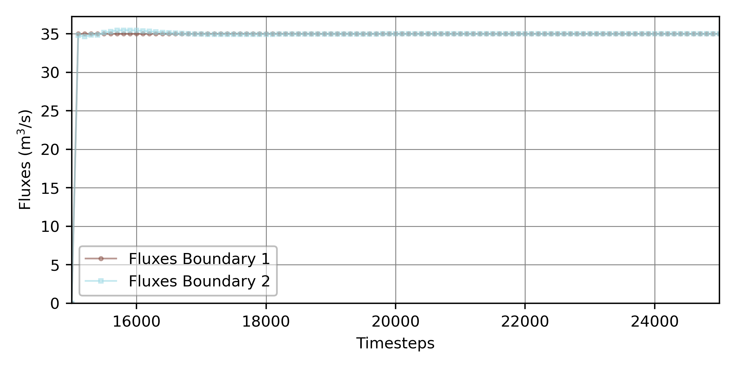
Figure 24:Flusskonvergenzkurve über die beiden Grenzen der stationären Telemac2d-Simulation mit Warmstart, beginnend bei einer Simulationszeit von 15000 Zeitschritten.
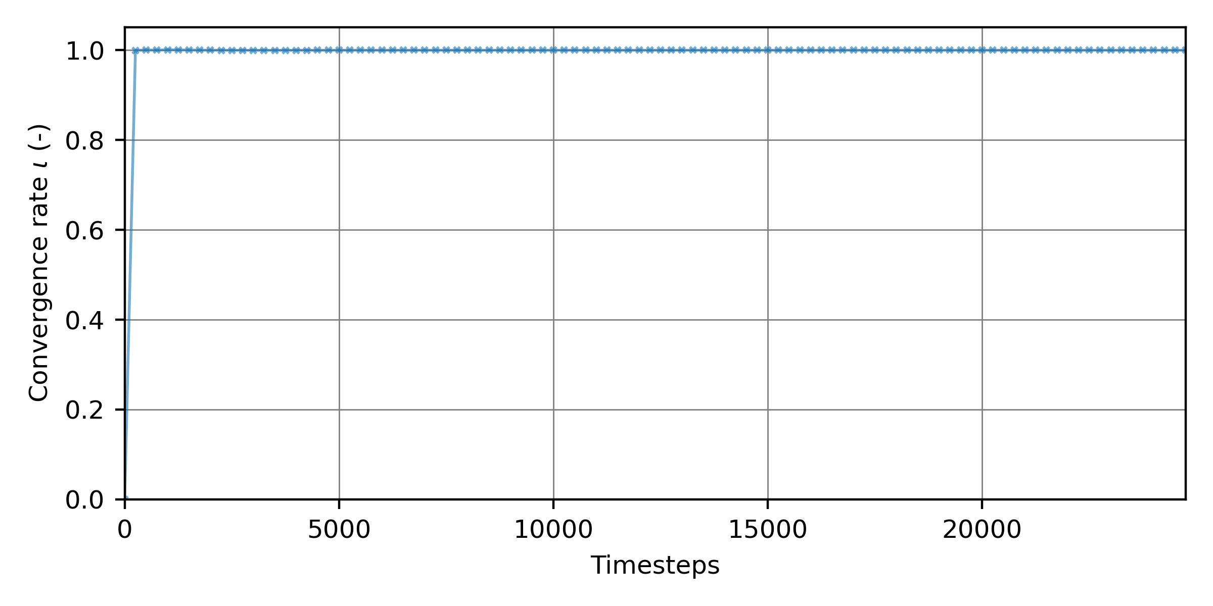
Figure 25:The convergence rate as a function 15000 simulation timesteps of the hotstarted steady 2d simulation with friction zones.
Die erforderliche steady2d-zonal-ks.cas 2023-07-28-14h55min04s ist hier verfügbar für die Verwendung mit Anweisungen aus dem Spotlight-Kapitel unter convergence.
Arbeiten mit Friction IDs
Die Reibungszonen können auch über Reibungs-IDs zugewiesen werden, die dann die Einrichtung einer Zonendatei und einer Reibungsdatendatei erfordern, wie im Donau-Beispiel (HOMETEL/examples/telemac2d/donau/) dargestellt.
In the showcase of this tutorial, working with friction tables required assigning the friction IDs defined in Tab. 1 to the BOTTOM FRICTION variable of the .slf mesh. The according files can be downloaded from our repositories:
Holen Sie sich Friction-with-IDs.xyz für Interpolation in BlueKenue (see above) oder direkt
get qgismesh-frictionIDs.slf with
BOTTOMandFRIC_IDinstead ofBOTTOM FRICTIONStrickler roughness coefficients (uses default friction ID0).
Reibung.tbl & CAS
Erstellen von friction.tbl
Erstellen Sie eine Friktionstabellendatei mit dem Namen friction.tbl (beachten Sie diese friction.tbl template]] mit folgendem Inhalt, wobei die no-Einträge (hier beginnend in Zeile 36) dem FRIC_ID entsprechen müssen, der dem Mesh zugewiesen ist (erinnern Sie sich an Fig. 20):
1 2 3 4 5 6 7 8 9 10 11 12 13 14 15 16 17 18 19 20 21 22 23 24 25 26 27 28 29 30 31 32 33 34 35 36 37 38 39 40 41* ----------------------------------------------------------------------------- * EXAMPLE ADAPTED FROM HOMETEL/examples/telemac2d/donau/ * * Implemented roughness laws: * NOFR : no friction (number of values) * HAAL : Haaland law (1 value : rB) * CHEZ : Chezy law (1 value : rB) * STRI : Strickler law (1 value : rB) * MANN : Manning law (1 value : rB) * NIKU : Nikuradse law (1 value : rB) * LOGW : Log Wall law (1 value : rB) * COWH : Colebrook-White law (2 values : rB, nDef) * * no : FRIC_ID assigned to the SLF mesh * * Riverbed * ------------- * typeB : roughness law for riverbed * rB : friction value for riverbed * nDefB : Mannings n for shallow flow zones * * Later walls (only with k-epsilon model) * ----------------------------------------- * typeS : roughness law for walls (option) * rS : friction value for walls (option) * nDefS : Mannings n for shallow waters (option) * * Non-submerged Vegetation (if needed) * ------------------------ * dp : mean diameter (option) * sp : averaged distance between roughness elements (option) * * ----------------------------------------------------------------------------- * no typeB rB NDefB typeS rS NDefS dp sp * 0 STRI 33.0 NULL 1 STRI 34.6 NULL 2 STRI 27.7 NULL 3 STRI 40.3 NULL 4 STRI 22.7 NULL END
Program 1:Example for a friction(.tbl) ID table.
Link friction.tbl in der CAS-Datei
To activate the friction data, add the following keywords to the .cas steering file, and deactivate any not-wall related FRICTION keywords:
/ steady2d-zonal-ks.cas steering file
/ ...
/ ACTIVATE these keywords
FRICTION DATA : YES / default is NO
FRICTION DATA FILE : 'friction.tbl'
MAXIMUM NUMBER OF FRICTION DOMAINS : 20 / consider to increase (default is 10)
/ steady2d-zonal-ks.cas steering file
/ ...
/ DEACTIVATE these keywords
/ LAW OF BOTTOM FRICTION : 3 / 3-Strickler
/ FRICTION COEFFICIENT : 80 / not use with zonal frictionSave the .cas steering file.
Ausführen von Telemac mit Friction IDs
To run Telemac with friction IDs, make sure the above-indicated keywords are activated in the .cas steering file. The required files now embrace:
qgismesh
-frictionIDs .slf (mesh mit FRIC_ID)]boundaries.cli oder Hotstartbedingungen]
r2dsteady-t15k.slfErgebnisdatei zum Aktivieren des Hotstarts]
steady2d
-zonal -ID .cas Steering-Datei aktualisierte Keywords] friction.tbl mit Reibungs-IDs]
Aktivieren und Ausführen von Telemac mit diesen Dateien wie gewohnt:
cd ~/telemac/v9.0.0/configs
source pysource.gfortranHPC.sh
cd ~/modeling/frictionID-tutorial/
telemac2d.py steady2d-zonal-ID.cas
Erweiterte Friktionsroutinen
Modifying the FRICTION_USER Fortran subroutines is not mandatory for working with friction zones but can be useful for implementing or adapting the behavior of roughness laws. To activate a FRICTION_USER subroutine, for example, to implement the variable power equation from Ferguson (2007):
Kopieren Sie die Subroutinevorlage FICTION USER von
HOMETEL/sources/telemac2d/friction_user.fin einen neuen Ordner Ihres Simulationsverzeichnisses, zum Beispiel:
/HOME/modeling/frictionID-tutorial/user_fortran/friction_user.fModify and save edits of
friction_user.f.Sagen Sie der Steuerungsdatei (
.cas), die modifizierte FRICTION USER Fortran-Datei zu verwenden, indem Sie das SchlüsselwortFORTRAN FILE : 'user_fortran'hinzufügen, wodurch Telemac2d Fortran-Dateien im/user_fortran/-Unterordner nachschlagen lässt.
- Díaz Gómez, R., Pasternack, G. B., Guillon, H., Byrne, C. F., Schwindt, S., Larrieu, K. G., & Solis, S. S. (2022). Mapping Subaerial Sand-Gravel-Cobble Fluvial Sediment Facies Using Airborne Lidar and Machine Learning. Geomorphology, 401, 108106. https://www.sciencedirect.com/science/article/pii/S0169555X21005146
- Google. (nd). Google Satellite Imagery. https://mt1.google.com/vt/lyrs=s&x=%7Bx%7D&y=%7By%7D&z=%7Bz%7D
- Meyer-Peter, E., & Müller, R. (1948). Formulas for Bed-Load transport. IAHSR, Appendix 2, 2nd meeting, 39–65. http://resolver.tudelft.nl/uuid:4fda9b61-be28-4703-ab06-43cdc2a21bd7
- Strickler, A. (1923). Beiträge zur Frage der Geschwindigkeitsformel und der Rauhigkeitszahlen für Ströme, Kanäle und geschlossene Leitungen [Contributions to the question of the velocity formula and the roughness figures for streams, channels and closed pipes]. Mitteilungen Des Eidgenössischen Amtes Für Wasserwirtschaft, Switzerland, 16, 357.
- Rickenmann, D., & Recking, A. (2011). Evaluation of flow resistance in gravel-bed rivers through a large field data set. Water Resources Research, 47, W07538. 10.1029/2010WR009793
- Ferguson, R. (2007). Flow resistance equations for gravel- and boulder-bed streams. Water Resources Research, 43, W05427. 10.1029/2006WR005422