Terminologie
Eine hydromorphodynamische Simulation impliziert die Modellierung von ablaufenden Sedimenttransport Prozessen. Die vorherigen Abschnitte in diesem eBook konzentrieren sich auf Hydrodynamik definiert als *die Untersuchung von Flüssigkeiten in Bewegung * und dieser Abschnitt konzentriert sich auf ** Morphodynamik * definiert als **die Untersuchung von zeitabhängigen Veränderungen in den Formen von Schwemmbetten und ihren zugrunde liegenden Prozessen *.
Sediment Transport Modi
TELEMAC has a dedicated module called Gaia for modeling morphodynamics. Gaia enables modeling sediment transport and morphological evolution (i.e., Topografischer Wandel) in rivers, lakes, and estuaries. It comes with particular routines to consider a spatio-temporal variation of grain sizes, grading curves, and riverbed layering for simulating sediment transport in the form of Geschiebe (coarse sediment) and/or Schwebstoff (fine sediment). Geschiebe is calculated by solving semi-empiric equations, such as the Meyer-Peter & Müller (1948) formula (read more later in this tutorial). Schwebstoff is modeled by solving the Advektion-Diffusion equations (typically, the RANS form), which require closures for sediment erosion and deposition fluxes. Figure 1 qualitatively illustrates the two basic modes of sediment transport in the form of suspended load and bedload. Whether a particle is transported in suspension or as bedload can also be determined by calculating of the Rouse number.
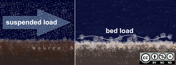
Figure 1:Qualitative Darstellung von zwei Arten des Sedimenttransports. Links: Schwebstofffracht in Form von feinen Partikeln, die sich mit dem Massenstrom bewegen; rechts: Geschiebefracht in Form von Partikeln, die auf dem Flussbett rollen, springen oder gleiten.
Sediment is further distinguished between very fine, cohesive sediment and coarser, non-cohesive sediment. In addition, Gaia accounts for bed evolution through an iterative solution of the Exner-Gleichung Exner, 1925 for mass conservation.
Die Rekrutierung von Sedimenten sowohl für die Schwebstofffracht als auch für den Bettentransport erfordert einen detaillierten Blick auf das Flussbett, der später im Abschnitt über die Definition von the riverbed composition and the active layer bereitgestellt wird.
Kopplung von TELEMAC und Gaia
Das Morphodynamikmodul Gaia kann intern mit den hydrodynamischen Modellen Telemac2d (auflösen des Flachwassergleichungen) oder Telemac3d (auflösen des Reynolds-gemittelten Navier-Stokes (RANS) equations) gekoppelt werden. In diesem Abschnitt werden Arten der Kopplung von Telemac2d/Telemac3d (Hydrodynamik) mit Gaia (Morphodynamik) erläutert.
Von Sisyphe zu Gaia
Sisyphe ist das traditionelle Sedimenttransportmodul in TELEMAC, das weitgehend durch das einheitlichere Gaia-Modul ersetzt wurde. Gaia basiert auf dem historischen Modul SISYPHE, mit einer Vielzahl von Verbesserungen, Korrekturen und Optimierungen. Gaias einheitliches Framework verwaltet effizient verschiedene Sedimentklassen, Sand-Schlamm-Mischungen und sowohl 2D- als auch 3D-Raumdimensionen. Um Spezifikationen zu erhalten, die über die hier in der TELEMAC-Dokumentation und im TELEMAC-Forum vorgestellten Funktionen hinausgehen, ist es nützlich, das SISYPHE-Erbe zu kennen. SISYPHE-Routinen sind immer noch in den letzten TELEMAC-Versionen über Gaia verfügbar, obwohl einige Keywords Anpassungen erfordern. Lesen Sie mehr im Gaia manual in Anhang 8.1 und im gaia.dico (telemac/v9.0.0/sources/gaia/gaia.dico).
Kupplung Hydrodynamik (Telemac2d/3d) und Morphodynamik (Gaia)
Ein hydromorphodynamisches numerisches Modell kann entweder **voll gekoppelt ** oder **entkoppelt ** werden.
- Fully coupled model
- A fully coupled model solves the hydrodynamic Navier-Stokes-Gleichungen simultaneously with sediment transport equations (i.e., erosion and deposition fluxes from and to the riverbed through the Exner-Gleichung). Bed elevation (i.e., Topografischer Wandel) is calculated for every timestep, which leads to long computation times. In addition to the coupling of gravity-driven hydrodynamics (i.e., bulk flow along valley slopes), Sedimenttransport, and Topografischer Wandel, a model can also be coupled with (surface) wave hydrodynamics.
Anwendungsbereich: Schnelle morphodynamische Prozesse wie hyperkonzentrierte sedimentbeladene Strömungen oder Trümmerströme.
- Decoupled model
- A decoupled model alternates between solving hydrodynamics and morphodynamics (i.e., the Exner-Gleichung). The riverbed is considered fixed when hydrodynamic variables are computed, and then bed elevation changes are calculated separately based on the computed flow field. This asynchronous approach is computationally more efficient than full coupling.
Anwendungsbereich: Die meisten Flussmodelle und insbesondere See- oder Ozeanmodelle, bei denen morphodynamische Zeitskalen viel länger sind als hydrodynamische Zeitskalen.
Gaia folgt dem **entkoppelten ** Ansatz. Der für die morphodynamische Berechnung verwendete Zeitschritt ist der gleiche wie für die Hydrodynamik (angegeben in der Telemac2d- oder Telemac3d-Lenkdatei). In jedem Zeitschritt wird die Hydrodynamik zuerst mit dem eingefrorenen Bett gelöst, dann werden die Sedimenttransportgleichungen und die Bettentwicklung (Exner-Gleichung) basierend auf dem berechneten Strömungsfeld gelöst.
Anforderungen an die Kupplung Gaia
In addition to the standard Telemac2d steering, boundaries, and geometry mesh files, coupling hydrodynamics with Gaia requires a new steering (*.cas) file that needs to be referenced in the main steering file of the simulation. To this end, create a new folder for the Gaia tutorial (e.g., called /gaia2d-tutorial/), copy the dry-initialized steady2d simulation and results files (or clone the gaia2d-tutorial repository), and create a new Gaia steering file (e.g., called gaia-morphodynamics.cas). Thus, the following files should live in the modeling folder for this tutorial:
Das Rechennetz in Form von qgismesh.slf].
Die Randdefinitionen in Form von boundaries.cli].
Die Ergebnisse des trocken-initialisierten stationären 2D-Modells laufen für 35 m/s in Form von r2dsteady.slf (dry steady runend bei
T=15000).Eine Telemac2d-Steuerungsdatei für dieses Tutorial, die auf der trocken initialisierten steady2d-Steuerungsdatei aufbaut und steady2d-gaia.cas] aufgerufen wird.
Die neue gaia
-morphodynamics .cas Steering-Datei].
Paar Gaia in der hydrodynamischen Lenkdatei
Um die Kopplung von Gaia mit einer Telemac2d/Telemac3d-Simulation programmatisch zu implementieren, müssen zusätzlich zu den im steady2d chapter erläuterten Keywords einige neue Keywords definiert werden. Das erste zusätzliche Schlüsselwort ist die Baseline für jede Kopplung mit Telemac2d oder Telemac3d Steuerungsdatei:
/ steady2d-gaia.cas
COUPLING WITH : 'GAIA'Darüber hinaus verknüpft das Schlüsselwort GAIA STEERING FILE das oben erstellte gaia-morphodynamics.cas in der Steuerungsdatei für die Hydrodynamik von Telemac2d (oder Telemac3d):
/ steady2d-gaia.cas
/ ...
GAIA STEERING FILE : gaia-morphodynamics.casHeißstart
This tutorial builds on the results of the dry-initialized steady2d model because Gaia simulations typically require a well-developed flow field as initial condition (see the above definitions). Using a former simulation result for model initialization is called hotstart, which requires a results file from a previous simulation. For this purpose, make sure that the dry-initialized steady2d results file is in the simulation folder (download r2dsteady.slf). Then define the hotstart in the Telemac2d steering file with the following keywords:
/ steady2d-gaia.cas
/ ...
PREVIOUS COMPUTATION FILE : r2dsteady.slf / results of 35 CMS steady simulation
INITIAL TIME SET TO ZERO : YES / avoid restarting at 15000Mit dem Schlüsselwort INIAL TIME SET TO NULL wird die Simulationszeit auf 0 zurückgesetzt. Stellen Sie als nächstes sicher, dass alle INITIAL BEDINGUNGEN-Keywords mit / kommentiert werden (alternativ löschen Sie diese Zeilen von steady2d-gaia.cas):
/ steady2d-gaia.cas
/ ...
/ INITIAL CONDITIONS - not required (hotstart)
/ ------------------------------------------------------------------
/ INITIAL CONDITIONS : 'ZERO DEPTH' / use ZERO DEPTH to start with dry model conditions
/ INITIAL DEPTH : 0.005 / use INTEGER for speeding up calculationsThe dry-initialized steering file prescribes flowrates and elevations, which requires modifications in steady2d-gaia.cas to prescribed Q only. The reason for the Q-only prescription is that with Gaia, we want to model-predict changes in water depths and riverbed elevation, which means that the water surface elevation must not be constrained (i.e., not prescribed) as a boundary condition. Thus, the setup of boundary conditions for Gaia also requires slight modifications of the boundary (*.cli) file(s), which will be explained in the next section on the Basic Setup of Gaia. To this end, make sure that in the hydrodynamics steering file only the flowrate prescription keyword is activated and the elevation prescription is deactivated (comment out with /):
/ steady2d-gaia.cas
/ ...
/ Liquid boundaries
PRESCRIBED FLOWRATES  : 35.;35.
/ PRESCRIBED ELEVATIONS : 374.805626;371.33Steuerabschnitte
Control sections are sequences of node numbers (or node coordinates) at which TELEMAC sums up fluxes, for instance, to verify inflow and outflow mass balances. The unsteady simulation section provides detailed instructions for defining control sections and this tutorial re-uses the control sections file from the unsteady simulation (download control-sections.txt).
Expand to view the file control-sections.txt
# control sections steady2d
2 -1
Inflow_boundary
144 32
Outflow_boundary
34 5
Um die Kontrollabschnitte für die Gaia-Simulation zu verwenden, fügen Sie der Hydrodynamik-Lenkdatei Folgendes hinzu:
/ steady2d-gaia.cas
/ ...
SECTIONS INPUT FILE :  control-sections.txt
SECTIONS OUTPUT FILE : r-control-flows.txt
Beim erneuten Ausführen der Simulation werden die Flüsse über die beiden definierten Kontrollabschnitte in eine Datei namens r-control-flows.txt geschrieben.
Hydrodynamische Lenkung Zusammenfassung
With the above adaptions and using a simulation length of 30000 timesteps (to observe morphodynamic evolution) with a graphical printout period of every 5000 timesteps (to reduce the output file size), the final hydrodynamic steering file should look like this:
/ steady2d-gaia.cas
/
TITLE : 'gaia2d steady'
/
/ HOTSTART - continuation is automatic when PREVIOUS COMPUTATION FILE is specified (v9.0+)
PREVIOUS COMPUTATION FILE : r2dsteady.slf / here - 35 CMS initialization after t 15000
INITIAL TIME SET TO ZERO : YES / avoid restarting at 15000
/
COUPLING WITH : 'GAIA'
GAIA STEERING FILE : gaia-morphodynamics.cas
/
/ DEFAULTS FROM STEADY2D
/
/------------------------------------------------------------------/
/     COMPUTATION ENVIRONMENT
/------------------------------------------------------------------/
/
BOUNDARY CONDITIONS FILE : boundaries.cli
GEOMETRY FILE            : qgismesh.slf
RESULTS FILE           : r2dsteady-gaia.slf
/
MASS-BALANCE : YES / activates mass balance printouts - does not enforce mass balance
VARIABLES FOR GRAPHIC PRINTOUTS : U,V,H,S,Q,F / Q enables boundary flux equilibrium controls
/
/ CONTROL SECTIONS
SECTIONS INPUT FILE :  control-sections.txt
SECTIONS OUTPUT FILE : r-control-flows.txt
/
/------------------------------------------------------------------/
/     GENERAL PARAMETERS
/------------------------------------------------------------------/
TIME STEP : 1.
NUMBER OF TIME STEPS : 30000
GRAPHIC PRINTOUT PERIOD : 5000
LISTING PRINTOUT PERIOD : 5000
/
/------------------------------------------------------------------/
/     NUMERICAL PARAMETERS
/------------------------------------------------------------------/
/ General solver parameters from section 7.1
DISCRETIZATIONS IN SPACE : 11;11
FREE SURFACE GRADIENT COMPATIBILITY : 0.1  / default 1.
ADVECTION : YES
/
/ FINITE ELEMENT SCHEME PARAMETERS - section 7.2.1 in the manual
/------------------------------------------------------------------
TREATMENT OF THE LINEAR SYSTEM : 2 / default is 2 - use 1 to avoid smoothened results
SCHEME FOR ADVECTION OF VELOCITIES : 14 / alternatively keep 1
SCHEME FOR ADVECTION OF TRACERS : 5
SCHEME FOR ADVECTION OF K-EPSILON : 14
IMPLICITATION FOR DEPTH : 0.55 / should be between 0.55 and 0.6
IMPLICITATION FOR VELOCITY : 0.55 / should be between 0.55 and 0.6
IMPLICITATION FOR DIFFUSION OF VELOCITY : 1. / v9p0 default
IMPLICITATION COEFFICIENT OF TRACERS : 0.6 / v9p0 default
MASS-LUMPING ON H : 1.
MASS-LUMPING ON VELOCITY : 1.
MASS-LUMPING ON TRACERS : 1.
/ MASS-LUMPING FOR WEAK CHARACTERISTICS : 1. / enabling leads to weak characteristics
SUPG OPTION : 0;0;2;2  / classic supg for U and V
/
/ SOLVER
/------------------------------------------------------------------
INFORMATION ABOUT SOLVER : YES
SOLVER : 1
/
/ TIDAL FLATS  - see section 7.5
TIDAL FLATS : YES
CONTINUITY CORRECTION : YES / default is NO
OPTION FOR THE TREATMENT OF TIDAL FLATS : 1
TREATMENT OF NEGATIVE DEPTHS : 2 / value 2 or 3 is required with tidal flats - default is 1
/
/ MATRIX HANDLING - see section 7.6
MATRIX STORAGE : 3 / default is 3
/
/ BOUNDARY CONDITIONS
/------------------------------------------------------------------
/
LAW OF BOTTOM FRICTION : 4 / 4-Manning
FRICTION COEFFICIENT : 0.03 / Roughness coefficient
/
/ Liquid boundaries
PRESCRIBED FLOWRATES  : 35.;35.
/ PRESCRIBED ELEVATIONS : 374.805626;0.
/
/ Type of velocity profile can be 1-constant normal profile (default) and (cli) 4-vector is proportional to root (water depth, only for Q)
VELOCITY PROFILES : 4;1
/
/ INITIAL CONDITIONS - not required (hotstart)
/ ------------------------------------------------------------------
/ INITIAL CONDITIONS : 'ZERO DEPTH' / use ZERO DEPTH to start with dry model conditions
/ INITIAL DEPTH : 0.005 / use INTEGER for speeding up calculations
/
/ STABILITY CONTROLS
/ ------------------------------------------------------------------
PRINTING CUMULATED FLOWRATES : YES
/
/------------------------------------------------------------------/
/     TURBULENCE
/------------------------------------------------------------------/
/
DIFFUSION OF VELOCITY : YES / default is YES
TURBULENCE MODEL : 3
/
&ETA- Meyer-Peter, E., & Müller, R. (1948). Formulas for Bed-Load transport. IAHSR, Appendix 2, 2nd meeting, 39–65. http://resolver.tudelft.nl/uuid:4fda9b61-be28-4703-ab06-43cdc2a21bd7
- Exner, F. M. (1925). Über die Wechselwirkung zwischen Wasser und Geschiebe in Flüssen [About the Interdependency of Water and Bed load in Rivers]. Akademie Der Wissenschaften in Wien, Math.-Naturw. Klasse, Sitzungsberichte, Abt. IIa, 134, 165–203.