Konvergenz (Quantitative) - Hydro-Informatics

Requirements

Ergänzen Sie die Telemac steady 2d tutorial (oder eine äquivalente stationäre Simulation).
Die Steuerungsdatei (.cas) muss die Schlüsselwörter MASS-BALANCE : YES und/oder PRINTING CUMULATED FLOWRATES : YES enthalten, die TELEMAC dazu veranlassen, die Massenflüsse über die Flüssigkeitsgrenzen in der Auflistung zu melden.
Die TELEMAC-Simulation muss mit der -sfahne ausgeführt werden (Details unten):

telemac2d.py [STUDY-NAME].cas -s

Eine Python (≥ 3.9)-Installation mit der numpy,pandas und matplotlib-Bibliotheken (see the Python installation guide);flusstools ist nicht erforderlich.

Alle in diesem Tutorial verwendeten Simulationsdateien können vom Hydro-informatics/telemac-Repository auf GitHub(siehe unten) heruntergeladen werden.

Goals & purpose

In diesem Kapitel wird ein quantitatives Verfahren zur Überprüfung der Flusskonvergenz einer *steady TELEMAC-Simulation und zur Bestimmung der Mindestsimulationsdauer (NUMBER OF TIME STEPS) vorgestellt, die zur Erreichung eines massensymmetrischen Zustands erforderlich ist. Eine solche Überprüfung wird empfohlen, bevor ein stetiges Ergebnis verwendet wird, um eine unsteady oder eine morphodynamic (sediment transport)-Simulation zu starten, da die Kalibrierung oder Weiterführung von einem nicht konvergierten Zustand eine transiente Vorspannung in alle nachfolgenden Berechnungen propagiert. Das gleiche Verfahren kann auch angewendet werden, um die Laufzeiten von Flutwellen zwischen einer vorgeschalteten und einer nachgeschalteten Grenze zu vergleichen.

Für Abhilfemaßnahmen zu einem nicht konvergierenden Modell wenden Sie sich an die spotlight chapter on mass conservation und überprüfen Sie, ob die liquid boundaries are well defined.

Dieses Kapitel verwendet die Simulationsdateien der Telemac steady 2d tutorial, mit einer geänderten Definition des Zeitschritts und der Ausgabeperioden:

/ steady2d-conv.cas
TIME STEP : 1.
NUMBER OF TIME STEPS : 10000
GRAPHIC PRINTOUT PERIOD : 50
LISTING PRINTOUT PERIOD : 50

Darüber hinaus wurde die Simulation mit der -s-Flagge neu ausgeführt, die die vollständige Auflistung an eine Datei namens [FILE-NAME].cas_YEAR-MM-DD-HHhMMminSSs.sortie im Simulationsverzeichnis schreibt:

telemac2d.py steady2d-conv.cas -s

Sowohl die Steuerung .cas als auch die .sortie Dateien können von den hydro-informatics.com Repositories heruntergeladen werden:

Daten extrahieren und überprüfen¶

Die TELEMAC Jupyter Notebook-Vorlagen (HOMETEL/notebooks/ > data manip/extraction/*.ipynb oder workshops/exo fluxes.ipynb) liefern Leitlinien für die Datenextraktion aus Simulationsergebnissen; die Templates stellen jedoch keinen direkt anwendbaren Rahmen für die Bewertung der Massenkonvergenz an den Grenzen in Abhängigkeit von NUMBER OF TIME STEPS. Zu diesem Zweck unterhält hydro-informatics.com das leichte Python-Paket pythomac (Version ≥ 3.0.0 wird hier beschrieben). Das Paket benötigt nur numpy, pandas und matplotlib (see the Python installation guide) und läuft außerhalb der TELEMAC Python-Umgebung. Zwei Installationsoptionen stehen zur Verfügung:

pip-install pythomac (recommended)

editable install from source

Installieren Sie das pythomac Paket aus dem Python Package Index:

pip install pythomac

Für Entwicklungszwecke klonen Sie das pythomac-Repository von GitHub und installieren Sie es im bearbeitbaren Modus:

git clone https://github.com/hydro-informatics/pythomac.git
pip install -e pythomac

Beachten Sie, dass seit Version 3.0.0 pythomac ein regelmäßiges Python-Paket mit In-Package-Importen ist; das Kopieren des pythomac/pythomac/ordners neben einer Simulation (dem Pre-3.0 Workflow) wird nicht mehr unterstützt.

Die zentrale Funktion ist pythomac.extract_fluxes(). Es ordnet die jüngste .sortie-Liste neben der Lenkdatei, parsiert die Lautstärkebilanz und den für jede Flüssigkeitsgrenze gedruckten signierten Fluss bei jedem Auflistungsdruck (beide die klassischen THERE IS n LIQUID BOUNDARIES und die TELEMAC v9 NUMBER OF LIQUID BOUNDARIES: Auflistungsformate werden erkannt) und schreibt in das Simulationsverzeichnis:

extracted-fluxes.csv - die Zeitreihe des Volumens in der Domäne und des Flusses über jede Flüssigkeitsgrenze; und
flux-convergence.png - ein Diagramm der Flussgrößen über die Simulationszeit (optional, plotting=True).

The function returns the extracted series as a pandas.DataFrame indexed by simulation time; the working directory of the calling process is not modified. The implementation can be inspected in flux_analyst.py on GitHub, and the complete API documentation is available at https://pythomac.readthedocs.io.

Um die Funktion anzuwenden, kopieren Sie den folgenden Code in ein neues Python-Skript namens z.B. example_flux_convergence.py, das sich im Verzeichnis befindet, in dem die trocken-initialisierte stationäre2d-Simulation lief (oder download example flux convergence.py):

# example_flux_convergence.py

from pathlib import Path
from pythomac import extract_fluxes

simulation_dir = str(Path(__file__).parents[1])
telemac_cas = "steady2d.cas"

fluxes_df = extract_fluxes(
    model_directory=simulation_dir,
    cas_name=telemac_cas,
    plotting=True
)

Führen Sie das Python-Skript von einem Terminal (oder Anaconda Prompt) im Simulationsverzeichnis aus:

python example_flux_convergence.py

Das Skript platziert im Simulationsordner:

die CSV-Datei extracted-fluxes.csv (download) und
das Flusskonvergence-Plot (flux-convergence.png) über die Modellgrenzen hinweg (siehe Fig. 1), das qualitativ anzeigt, dass die Flußmittel nach ca. 6000-7000 Zeitschritten auf Konvergenz angegangen sind.

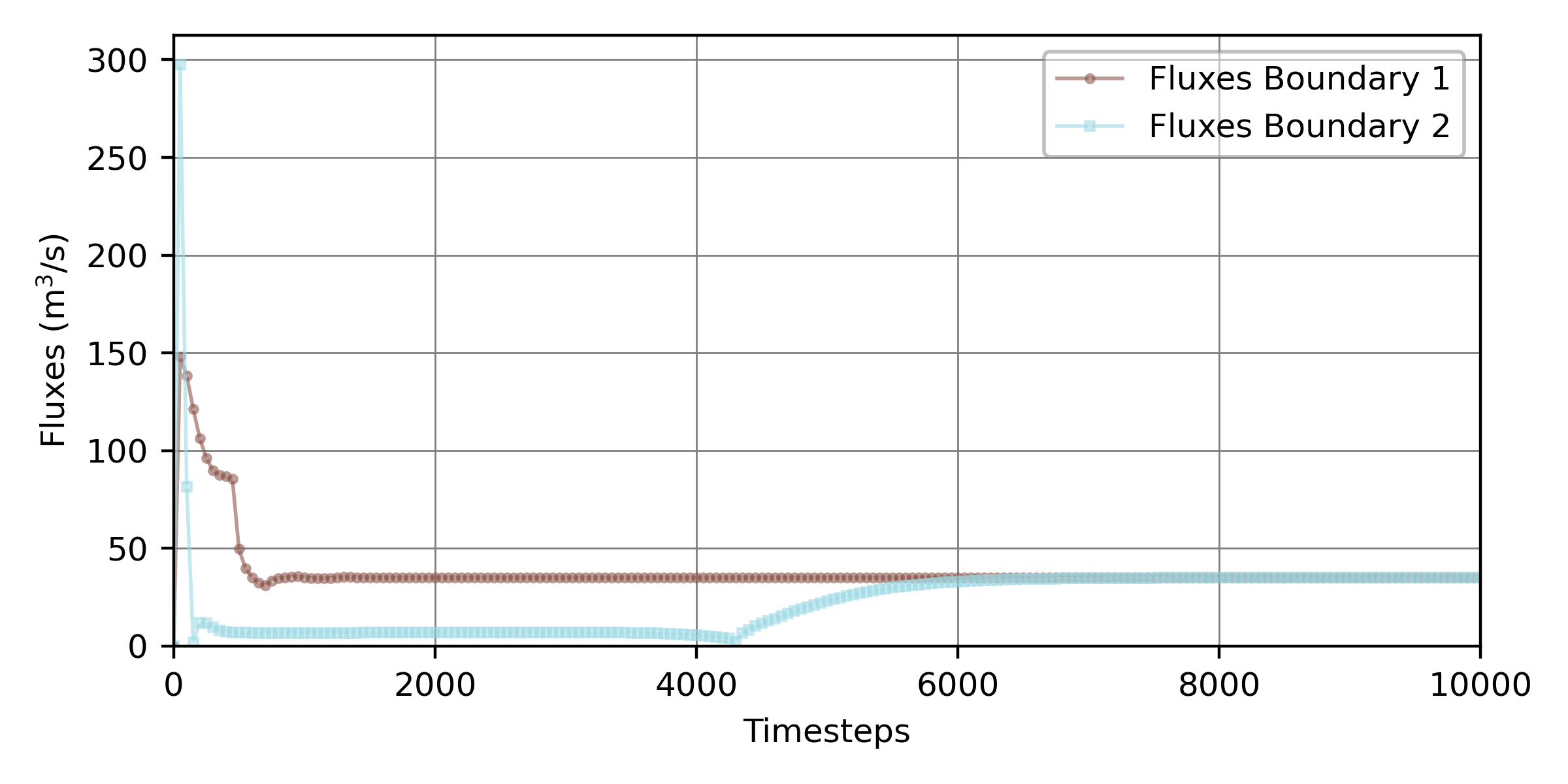
python telemac flux discharge convergence pythomac — Figure 1:Fluxgrößen über die beiden Flüssigkeitsgrenzen der trocken-initialisierten stationären Telemac2d-Simulation über die simulierte Zeit, die mit der pythomac.extract fluxes()-Funktion erzeugt wird.

Konvergence identifizieren¶

Um zu beurteilen, ob und wann die Grenzflüsse konvergiert werden, wird die relative Flussungleichgewichte zu jeder Druckzeit $t$ als:

\varepsilon_{t} = \frac{\left| |Q_{i,t}| - |Q_{j,t}| \right|}{|Q_{j,t}|}

(1)

wobei $Q_{i,t}$ und $Q_{j,t}$ = der Abfluss und der Zufluss über die Modellgrenzen hinweg zum Zeitpunkt $t$ bzw. Die Flussgrößen $|\cdot|$ sind erforderlich, weil TELEMAC Grenzflüsse mit einer Vorzeichenkonvention meldet (Zufluss positiv, Abflussnegativ); Massenbilanz entspricht daher $|Q_{i,t}| = |Q_{j,t}|$ , so dass $\varepsilon_{t} \to 0$ at Konvergenz und Normalisierung durch den Zufluss $|Q_{j,t}|$ renders $\varepsilon_{t}$ dimensionslos. In einer stabilen stetigen Simulation nähert sich das Verhältnis aufeinanderfolgender Flussungleichgewichte einer Konvergenzkonstanten $c_{\varepsilon}$ gleich der Einheit mit zunehmender Zeit:

\lim_{t\to \infty} \frac{\varepsilon_{t+1}}{\varepsilon^{\iota}_{t}} = c_{\varepsilon}

(2)

Die Kombination der Konvergenzrate (oder Bestellung) $\iota$ und der Konvergenzkonstante $c_{\varepsilon}$ gibt an:

lineare Konvergenz, wenn $\iota$ = 1 ** und** $c_{\varepsilon} \in ]0, 1[$
langsam sublinear Konvergenz, wenn $\iota$ = 1 ** und** $c_{\varepsilon}$ = 1;
schnelle superlinear Konvergenz, wenn $\iota$ > 1 ** und** $c_{\varepsilon} \in ]0, 1]$ und
Divergenz, wenn $\iota$ = 1 ** und** $c_{\varepsilon}$ > 1, ** oder* $\iota$ < 1.

Calculate

\varepsilon_{t+1}

$\varepsilon_{t+1}$ (epsilon_t1) wird von $\varepsilon_{t}$ (epsilon_t0) erhalten, indem die Serie um ein Element verschoben wird:

epsilon_t0 = epsilon[:-1]  # cut off last element
epsilon_t1 = epsilon[1:]   # cut off element zero

Die Zeit, zu der eine stetige Simulation als stabiler Zustand betrachtet werden kann, wird durch den Beginn der sublinearen Konvergenz ( $\iota$ = 1 und $c_{\varepsilon}$ = 1) ermittelt, d.h. die Zeit $t$ , über die jeder zusätzliche Schritt $t+1$ die Modellgenauigkeit nur unwesentlich verbessert (der Begriff insignificant wird in der section below quantifiziert). Unter der Annahme, dass das Modell in irgendeiner Form konvergiert, ergibt die Einstellung $c_{\varepsilon}$ = 1 $\iota(t)$ in Abhängigkeit von $\varepsilon_{t}$ und $\varepsilon_{t+1}$ :

\begin{align} \label{estimate convergence} ^^^^^^^^^^^^^^^^^^^^^^^^^^^^^^^^^^^^^^^^^^^^^^^^^^^^^^^^^^^^^^^^^^^^^^^^^^^^^^^^^^^^^^^^^^^^^^^^^^^^^^^^^^^^^^^^^^^^^^^^^^^^^^^^^^^^^^^^^^^^^^^^^^^^^^^^^^^^^^^^^^^^^^^^^^^^^^^^^^^^^^^^^^^^^^^^^^^^^^^^^^^^^^^^^^^^^^^^^^^^^^^^^^^^^^^^^^^^^^^^^^^^^^^^^^^^^^^ (c {\varepsilon} ^^^^^^^^^^^^^^^^^^^^^^^^^^^^^^^^^^^^^^^^^^^^^^^^^^^^^^^^^^^^^^^^^^^^^^^^^^^^^^^^^^^^^^^^^^^^^^^^^^^^^^^^^^^^^^^^^^^^^^^^^^^^^^^^^^^^^^^^^^^^^^^^^^^^^^^^^^^^^^^^^^^^^^^^^^^^^^^^^^^^^^^^^^^^^^^^^^^^^^^^^^^^^^^^^^^^^^^^^^^^^^^^^^^^^^^^^^^^^^^^^^^^^^^^^^^^^^^ \iota(t) &= \log {\varepsilon {t}\varepsilon {t+1} & (Ausrichtung)

Diese Beziehungen werden in der pythomac.calculate_convergence()-Funktion umgesetzt, die eine pandas.DataFrame mit den Spalten "Relative imbalance" ( $\varepsilon_{t+1}$ , Equation(1)) und "Convergence rate" ( $\iota(t)$ ) zurückgibt. Sein Kern lautet:

import numpy as np
import pandas as pd


def calculate_convergence(series_1, series_2, conv_constant=1.):
    # relative flux imbalance epsilon_t = ||Q_in| - |Q_out|| / |Q_in|; the magnitudes |.|
    #   are needed because Telemac reports outflow negative, so that balance -> epsilon -> 0
    epsilon = np.abs(np.abs(series_1) - np.abs(series_2)) / np.abs(series_1)
    # derive epsilon at t and t+1
    epsilon_t0 = epsilon[:-1]  # cut off last element
    epsilon_t1 = epsilon[1:]   # cut off element zero
    # return the relative imbalance and the convergence rate iota as a pandas DataFrame
    return pd.DataFrame({
        "Relative imbalance": epsilon_t1,
        "Convergence rate": np.emath.logn(epsilon_t0, epsilon_t1) / conv_constant,
    })

This function is available in pythomac

from pythomac import calculate_convergence

Die verpackte Implementierung akzeptiert zusätzlich cas_timestep (die Ausdruckabstände in Simulationsssekunden, die zur Skala des Index verwendet werden) und plot_dir (falls vorhanden, wird ein convergence-rate.png-Plot an dieses Verzeichnis geschrieben).

Um $\iota(t)$ (Python variabler Name: iota_t) mit der obigen Funktion zu berechnen, ändern Sie die example flux convergence.py Python Skript wie folgt:

# example_flux_convergence.py

# ...
# add to header:
from pythomac import calculate_convergence

# calculate fluxes_df (see above code block)
fluxes_df = [...]

# back-calculate the printout spacing (in simulation seconds) from the flux index
timestep_in_cas = int(max(fluxes_df.index.values) / (len(fluxes_df.index.values) - 1))

# calculate iota (t) with the calculate_convergence function
iota_t = calculate_convergence(
    series_1=fluxes_df["Fluxes Boundary 1"][1:],  # remove first zero-entry
    series_2=fluxes_df["Fluxes Boundary 2"][1:],  # remove first zero-entry
    cas_timestep=timestep_in_cas,
    plot_dir=simulation_dir,
)

Die daraus resultierende Konvergenzrate $\iota(t)$ ist in Fig. 2 für die steady 2d tutorial mit den geänderten Ausdrucksperioden von 50Sek. und einer Gesamtsimulationszeit von 10000Sek. aufgetragen.

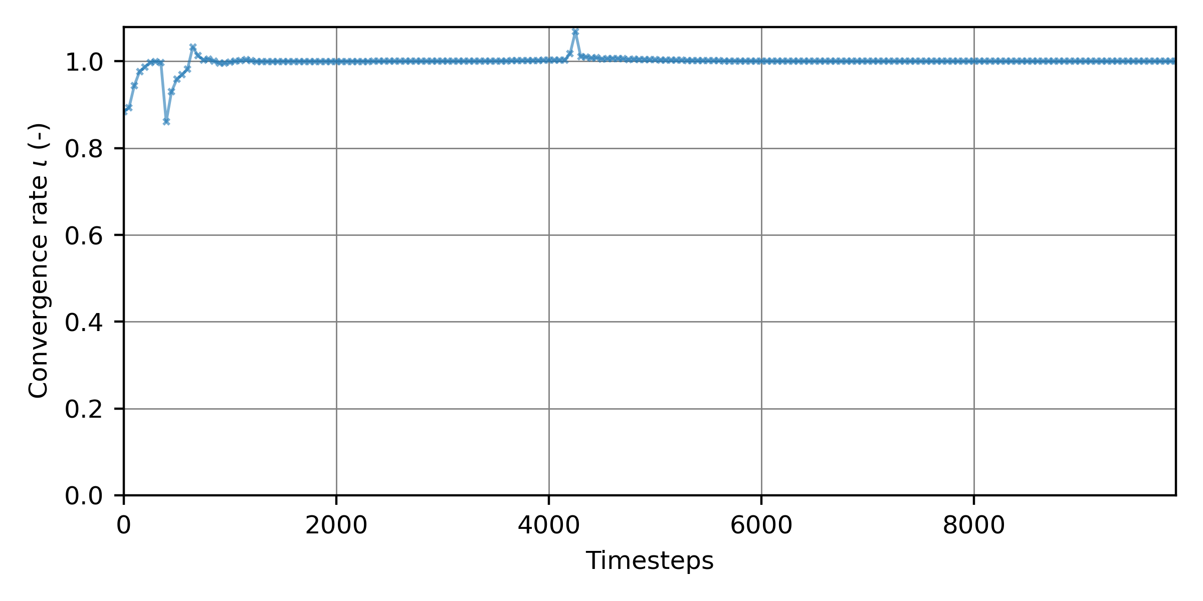
convergence rate fluxes telemac boundaries — Figure 2:Die Konvergenzrate $\iota$ in Abhängigkeit von den 10000 Simulationszeitschritten der stationären 2d-Simulation.

Abwechslungsreiche Simulationszeit¶

Um die Rechenzeit zu berechnen, ist der Zeitschritt, zu dem die Zu- und Abflüsse zusammenfließen, von praktischem Interesse. Die in Fig. 1 und der Konvergenzrate in Fig. 2 erstellten Flußmittel legen qualitativ nahe, dass die Simulation nach ca. 6000 Sekunden stabilisiert ist (Zeitschritte). Die lokale Extrema in beiden Figuren in der Nähe von 4000 Zeitschritten markieren die Wechselwirkung der Netzfronten, die sich von den vor- und nachgelagerten Grenzen ausbreiten (siehe animation in the steady 2d tutorial); monotone Konvergenz setzt erst danach ein.

Da ein rein visuelles Konvergenzurteil subjektiv ist, wird ein objektives Kriterium angenommen: Die optimale Simulationslänge ist die kleinste Zeit $t$ , über die das relative Flussungleichgewicht $\varepsilon_{t}$ (Equation (1)) dauerhaft unter einer Zieltoleranz $\varepsilon_{tar}$ bleibt. Toleranzen von $\varepsilon_{tar}$ = 10 $^{-4}$ sind in der Regel für Vorkalibrierungen akzeptabel, während Validierung und Hotstart-Initialisierung kleinere Werte (10 $^{-6}$ oder kleiner) garantieren. Wie Fig. 2 illustriert, kann das Ungleichgewicht vorübergehend unter die Toleranz fallen und wieder ansteigen (hier bei 4000 Zeitschritten, wenn die vorgeschaltete Front die nachgeschaltete Grenze passiert); nur die endgültige, dauerhafte Überquerung ist relevant. Die algorithmische Umsetzung erfasst daher das letzte Mal, bei dem $\varepsilon_{t} \geq \varepsilon_{tar}$ den nachfolgenden Ausdruck als Konvergenzzeit bezeichnet. Dieses Kriterium wird in pythomac.get_convergence_time(), die den Ausdrucksindex der Dauerüberfahrt zurückgibt, oder numpy.nan (mit Warnung) umgesetzt, wenn die Toleranz niemals erhalten bleibt. Das Skript example flux convergence.py wie folgt ändern:

# example_flux_convergence.py

# ...
# add to header:
from pythomac import get_convergence_time

# calculate fluxes_df and iota_t (see above code blocks)
fluxes_df = [...]
iota_t = [...]

# identify the printout index from which the relative flux imbalance stays
# permanently below the target tolerance (epsilon_tar)
convergence_time_iteration = get_convergence_time(
    relative_imbalance=iota_t["Relative imbalance"],
    convergence_precision=1.0E-4
)

if not str(convergence_time_iteration).lower() == "nan":
    print("The simulation converged after {0} simulation seconds ({1}th printout).".format(
            str(timestep_in_cas * convergence_time_iteration), str(convergence_time_iteration)))

The simulation converged after 6000 simulation seconds (120th printout).

Mit der festgelegten Konvergenzzeit kann das NUMBER OF TIME STEPS Schlüsselwort in der .casLenkungsdatei entsprechend reduziert werden, beispielsweise:

/ steady2d-conv.cas
TIME STEP : 1.
NUMBER OF TIME STEPS : 6000
GRAPHIC PRINTOUT PERIOD : 50
LISTING PRINTOUT PERIOD : 50

Fehlerbehebung Instabilitäten & Divergenz¶

Wenn eine stetige Simulation keine stabilen Flußmittel erreicht, oder wenn die Flußmittel divergieren, überprüfen Sie, ob alle Grenzen gemäß der Spotlight-Sektion auf boundary conditions robust definiert sind und konsultieren Sie den Workflow in der Rubrik mass conservation.