Run Gaia
Make sure that the simulation folder (e.g., /gaia2d-tutorial/) contains at least the following files (or similar, depending on the simulation case):
Ein Rechennetz, zum Beispiel in Form von qgismesh.slf].
Eine hydrodynamische Grenzdefinitionsdatei, zum Beispiel in Form von boundaries.cli].
Eine Gaia-Grenzendefinition, zum Beispiel in Form von boundaries-gaia.cli].
Eine Ergebnisdatei einer Telemac2d/3d-Simulation für eine Hotstart-Initialisierung, zum Beispiel für 35 m/s in Form von r2dsteady.slf] (Ergebnis der dry-initialized steady run-Endung bei
t=15000).Eine Telemac2d-Steuerungsdatei wie steady2d-gaia.cas].
Eine Gaia-Steuerungsdatei wie gaia
-morphodynamics .cas].
Expand to review the Gaia steering file gaia-morphodynamics.cas
/------------------------------------------------------------------/
/ Gaia in TELEMAC
/ GAIA STEERING FILE
/ file name: gaia-morphodynamics.cas
/
/------------------------------------------------------------------/
/                    COMPUTATION ENVIRONMENT
/------------------------------------------------------------------/
/
BOUNDARY CONDITIONS FILE : boundaries.cli
GEOMETRY FILE : qgismesh.slf
RESULTS FILE : rGaia-steady2d.slf
VARIABLES FOR GRAPHIC PRINTOUTS : B,E,M,MU,N,P,QSBL,TOB
MASS-BALANCE : YES
/
/ NUMERICAL OPTIONS
/------------------------------------------------------------------/
FINITE VOLUMES : NO
/------------------------------------------------------------------/
/
/------------------------------------------------------------------/
/ RIVERBED COMPOSITION
/------------------------------------------------------------------/
/
/ SEDIMENT
CLASSES TYPE OF SEDIMENT : NCO;NCO;NCO / CO-cohesive or NCO-non-cohesive
CLASSES SEDIMENT DIAMETERS : 0.0005;0.02;0.1 / in m
CLASSES SEDIMENT DENSITY : 2680;2680;2680 / in kg per m3
/
/ RIVERBED LAYERS - manual section 3.2.1
ACTIVE LAYER THICKNESS : 0.3 / multiple of D90 - default is 10000
NUMBER OF LAYERS FOR INITIAL STRATIFICATION : 3 / default is 1
LAYERS INITIAL THICKNESS : 1.5 / m - default is 100
/
/------------------------------------------------------------------/
/ BEDLOAD
/------------------------------------------------------------------/
/
/ BOUNDARIES
PRESCRIBED SOLID DISCHARGES : 10.;0.
/
BED LOAD FOR ALL SANDS : YES / deactivate with NO
BED-LOAD TRANSPORT FORMULA FOR ALL SANDS : 1 / MPM - see table for more
CLASSES SHIELDS PARAMETERS : 0.047;0.047;0.047
MPM COEFFICIENT : 8
/
/ BEDLOAD DIRECTION - manual sec. 3.1.4-3.1.7
SLOPE EFFECT : YES / default is YES - set to NO to disable
FORMULA FOR DEVIATION : 1 / use 2 for talmon-1995 approach
FORMULA FOR SLOPE EFFECT : 1 / default is 1 (koch-flokstra) change to 2 for soulsby
BETA : 1.3 / only with koch-flokstra - default is 1.3
/
/ SECONDARY CURRENTS - manual sec. 3.1.7
SECONDARY CURRENTS : YES / default is NO
SECONDARY CURRENTS ALPHA COEFFICIENT : 0.8 / default is 1.
/
/ FRICTION
SKIN FRICTION CORRECTION : 1 / set 0 to disable correction in shallow waters
RATIO BETWEEN SKIN FRICTION AND MEAN DIAMETER : 3. / default is 3.
/
/------------------------------------------------------------------/
/ SUSPENDED LOAD
/------------------------------------------------------------------/
/
SUSPENSION FOR ALL SANDS : YES / deactivate with NO
/
SUSPENSION TRANSPORT FORMULA FOR ALL SANDS : 1
/
/ NUMERICAL PARAMETERS
SCHEME FOR ADVECTION OF SUSPENDED SEDIMENTS : 14
/
/ ADDITIONAL SEDIMENT - manual section 4.2
CLASSES SETTLING VELOCITIES : -9;-9;-9 / use Gaia defaults
CLASSES CRITICAL SHEAR STRESS FOR MUD DEPOSITION : 1000;1000;1000 / N per m2
LAYERS PARTHENIADES CONSTANT : 1.E-03 / in kg per m2 per s - default is 1.E-03
With these files available, open Terminal, go to the TELEMAC configuration folder (e.g., ~/telemac/v9.0.0/configs/), and load the environment (e.g., pysource.openmpi.sh - use the same as for compiling TELEMAC).
cd ~/telemac/v9.0.0/configs
source pysource.openmpi.sh
Environment loading varies by installation
Der genaue Befehl zum Laden der TELEMAC-Umgebung hängt von Ihrer Installationskonfiguration ab. Gemeinsame Variationen umfassen:
Standardinstallation:
source pysource.openmpi.shodersource pysource.gfortran.shIntel-Compiler:
source pysource.intel.shCustom configurations: Check your
configs/folder for availablepysource.*.shfiles
If you encounter module loading errors, verify that all required dependencies (Python, MPI, compilers) are properly installed and configured. Refer to the TELEMAC installation guide for troubleshooting.
With the TELEMAC environment loaded, change to the directory where the TELEMAC Gaia simulation lives (e.g., /home/telemac/v9.0.0/mysimulations/gaia2d-tutorial/) and run the *.cas file by calling it with the telemac2d.py script (it will automatically know that it needs to use Gaia when it reads the line COUPLING WITH : 'GAIA').
cd ~/telemac/v9.0.0/mysimulations/gaia2d-tutorial/
telemac2d.py steady2d-gaia.casCommon runtime errors and solutions
Fehler: “STOP CALLED - ERHÖHEN ARRAY SIZE”
Ursache: Unzureichende Speicherzuweisung für das Mesh oder die Variablen
Lösung: Verringern Sie die Maschengröße oder erhöhen Sie den verfügbaren Speicher; Überprüfen Sie die Maschenqualität
Fehler: “NEGATIVE WATER DEPTH”
Ursache: Numerische Instabilitäten, oft aus zu großen Zeitschritten oder schlechter Mesh-Qualität
Lösung: Reduzieren Sie
TIME STEP, aktivieren SieTREATMENT OF NEGATIVE DEPTHS : 2, verbessern Sie die Maschenqualität in Problembereichen
Fehler: “SOLVER NOT CONVERGED”
Ursache: Linearer Solver hat das Konvergenzkriterium nicht erreicht
Lösung: Erhöhen Sie
MAXIMUM NUMBER OF ITERATIONS FOR SOLVER, entspannen SieSOLVER ACCURACYoder überprüfen Sie die Randbedingungen
Fehler: “FLOATING POINT EXCEPTION”
Ursache: Division durch Null oder Überlauf, oft aus sehr kleinen Wassertiefen
Lösung: Erhöhen Sie
MINIMAL VALUE OF THE WATER HEIGHT, überprüfen Sie die Anfangsbedingungen
Gaia-spezifisch: “NEGATIVE KONZENTRATION”
Ursache: Numerische Instabilitäten im Advektionsschema
Lösung: Verwenden Sie das Schema
14oder15für suspendierte Sedimente, reduzieren Sie den Zeitschritt, überprüfen Sie die Randbedingungen für Schwebstofffracht
Eine erfolgreiche Berechnung sollte mit den folgenden Zeilen (oder ähnlich) in *Terminal * enden:
[...]
                    *************************************
                    *    END OF MEMORY ORGANIZATION:    *
                    *************************************

CORRECT END OF RUN

ELAPSE TIME :
                             1  HOURS
                             4  MINUTES
                            34  SECONDS
... merging separated result files

... handling result files
       moving: r2dsteady-gaia.slf
       moving: rGaia-steady2d.slf
       moving: r-control-sections.txt
... deleting working dir

My work is done
TELEMAC schreibt die Dateien r2dsteady-gaia.slf, rGaia-steady2d.slf und r-control-sections.txt in den Simulationsordner. Diese Ergebnisdateien sind auch im Modellierungs-Repository dieses eBooks verfügbar, um das Nachbearbeitungs-Tutorial durchzuführen:
Download r2dsteady-gaia.slf (Hydrodynamik-Ergebnisse)]
Download rGaia-steady2d.slf(Morphodynamik-Ergebnisse)]
Download r-control-sections.txt (Steuerabschnittsflüsse)]
Nachbearbeitung
Regelstrecke Flussmittel
The control sections enable insights into the correct adaptation of the flow at the upstream and downstream boundaries (prescribed Q only). Figure 1 shows the modeled flow rates where the Inflow_boundary and Outflow_boundary curves converge after approximately 10000 timesteps. Note that the graph shows absolute numbers while the original output in r-control-sections.txt is negative because of the order of node definitions in control-sections.txt. The hotstart initialization makes that the fluxes fluctuate around the prescribed inflow of 35 m/s from the beginning. The Outflow_boundary flowrate increase toward the end of the simulation can be attributed to sediment erosion and the free flux downstream boundary type (544-4).
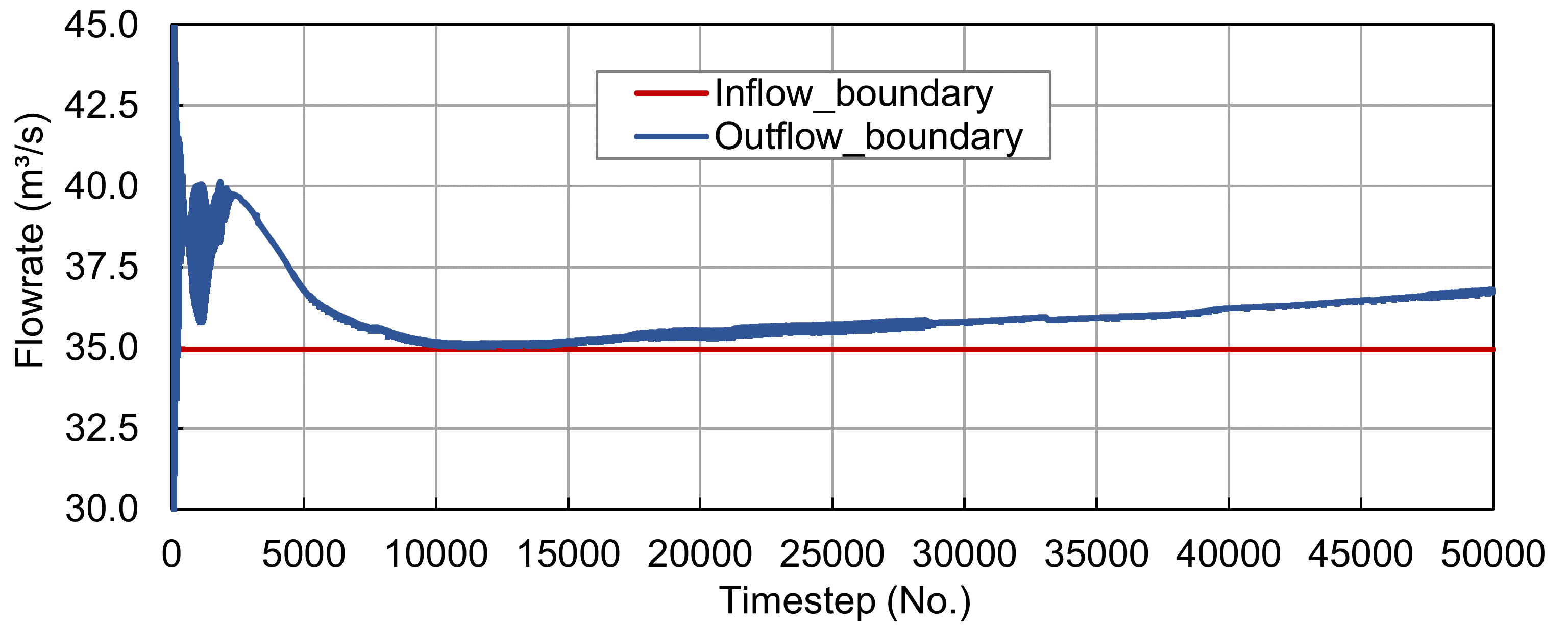
Figure 1:Die simulierten Flüsse fließen über die stromaufwärtigen Inflow boundary und die stromabwärtigen Outflow boundary Steuerabschnitte.
Visualisierung mit QGIS
The results of the Gaia simulation can be visualized and time snapshots exported to raster (e.g., GeoTIFF) or shapefile formats by using the PostTelemac plugin in QGIS the same way as explained in the steady2d tutorial. The latest QGIS releases additionally enable loading of a Selafin (results) mesh file (here: r2dsteady-gaia.slf) as QGIS mesh layer, which can then be visualized in the viewport and exported to a video with the Crayfish plugin. To this end, launch QGIS, set the project CRS to EPSG:25833 (ETRS89 / UTM zone 33N), and save the new project in the gaia2d-tutorial/ folder (or where ever the Gaia simulation files live). In QGIS’ Browser panel, find the Project Home folder, expand it, and drag-and-drop the two simulation results meshes (r2dsteady-gaia.slf and rGaia-steady2d.slf) to the Layers panel.
Doppelklicken Sie auf r2dsteady-gaia.slf oder rGaia-steady2d.slf, um ihre Mesh Layer Properties zu öffnen, und gehen Sie dann auf die Registerkarte Source, um hydrodynamische (z. B. Wassertiefe * oder * skalare Durchflussrate m2s) oder morphodynamische Gaia (z. B. * qs bedload kg(ms)*) Simulationsparameter in verschiedenen Zeitschritten umzuschalten. Figure 2 zeigt das QGIS-Mesh Layer Properties-Fenster der rGaia-steady2d.slf-Simulationsergebnisse Geometrie, in der rote Kästchen Schritte zum Umschalten von Ausgabevariablen und Visualisierungszeitschritten markieren. Darüber hinaus bietet die Registerkarte Symbology Optionen für Wertfarbenskalen oder Vektordarstellungen (z. B. für Geschwindigkeitsvektoren in r2dsteady-gaia.slf).
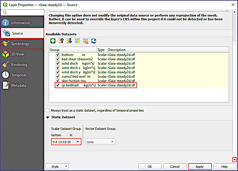
Figure 2:Das Mesh Layer Properties Fenster mit der Registerkarte Source zum Auswählen von Gaia-Ausgabevariablen. Der Screenshot zeigt Schritte zur Visualisierung von qs bedload zur Simulationsendzeit an (rote Boxen). Darüber hinaus können Plot-Farbbereiche in der Registerkarte Symbology (gestrichelte rote Box) angepasst werden.
rGaia-steady2d.slf (results file) not correctly showing in QGIS
Wird die Ergebnisdatei rGaia-steady2d.slf nicht in QGIS angezeigt? Importieren Sie es mit der korrekten Georeferenz: EPSG:25833 (ETRS 89 / UTM Zone 33N). Wenn das Netz an der falschen Stelle oder mit verzerrter Geometrie erscheint, ist Folgendes zu überprüfen:
Das Projekt Koordinatenreferenzsystem entspricht dem Mesh Koordinatenreferenzsystem (EPSG:25833)
On-the-fly-Reprojektion ist aktiviert, wenn ein anderes Projekt-Koordinatenreferenzsystem verwendet wird
Die ursprüngliche Geometriedatei verwendete das korrekte Koordinatenreferenzsystem
Um das Layer Koordinatenreferenzsystem manuell einzustellen: Rechtsklicken Sie auf die Layer → Set Koordinatenreferenzsystem → Set Layer Koordinatenreferenzsystem... → Suche nach EPSG:25833.
Beachten Sie, dass nur Parameter, die mit den Schlüsselwörtern VARIABLES FOR GRAPHIC PRINTOUTS in den Steuerungsdateien hydrodynamische (steady2d-gaia.cas) und morphodynamische (gaia-morphodynamics.cas) definiert sind, in QGIS aufgezeichnet werden können.
Um ein Video der Simulationsergebnisse zu exportieren, verwenden Sie das Plugin Crayfish:
Stellen Sie in QGIS sicher, dass das Crayfish-Plugin installiert ist (rufen Sie QGIS instructions zurück).
Wählen Sie im Feld Layer rGaia-steady2d (oder r2dsteady-gaia).
Mit rGaia-steady2d (oder r2dsteady-gaia) ausgewählt, gehen Sie zu Mesh (Top Dropdown-Menü) > Crayfish Export-Animation ... (wenn die Ebene nicht hervorgehoben ist, erscheint eine Fehlermeldung: Bitte wählen Sie eine Mesh-Ebene für den Export).
Gehen Sie im Fenster Export Animation zur Registerkarte Allgemein und definieren Sie einen Ausgabedateinamen, indem Sie auf die Schaltfläche ... klicken (z. B.
velocity-video.avi).Optional die Einstellungen Layout und Video anpassen.
Klicken Sie auf OK, um den Videoexport zu starten.
Beim ersten Export eines Videos benötigt Crayfish die Definition eines FFmpeg-Video-Encoders und führt durch die Installation (falls erforderlich). Befolgen Sie die Anweisungen und starten Sie den Export des Videos erneut. Das folgende Video wurde mit Crayfish exportiert, um Geschwindigkeitsvektoren zu visualisieren:
Video: Sebastian Schwindt @ Hydro-Morphodynamics channel on YouTube.
Beachten Sie, wie sich die Geschwindigkeitsvektoren im Laufe der Zeit entwickeln und dass hohe Strömungsgeschwindigkeiten an Rampen / Schwellen im Flussabschnitt auftreten (z. B. die beiden transversalen Maxima nahe der stromaufwärtigen Grenze oder das transversale Maximum nahe der stromabwärtigen Grenze). Dementsprechend sollte auch der Bettentransport an den Rampen ausgeprägt sein. Das folgende Video zeigt qs bedload, um zu überprüfen, ob das Modell die physikalische Verbindung zwischen Strömungsgeschwindigkeit und Geschiebefracht richtig hat.
Video: Sebastian Schwindt @ Hydro-Morphodynamics channel on YouTube.
After watching the video, it can be concluded that the relationship between flow velocities and bedload is approximately correct, but the model may require some correction by adapting magnitude and direction parameters. The next section exemplarily illustrates how the physical soundness of the model can be analyzed and improved.
Plausibilität
The above-shown results feature steady-state bedload and suspended load transport in an armored-bed river section at a low baseflow discharge of 35 m/s. The comparison of the flow velocity and the sediment transport videos suggests that the highest sediment transport rates occur where the flow velocity is high, too. Three sediment size classes were defined in the Basic Setup of Gaia with average grain diameters of 0.0005 m, 0.02 m, and 0.1 m. The simulation predicts that only the finest grain size class will move at baseflow (e.g., in the console output during the simulation). This fine sediment class of 0.5-mm diameters (sand) is transported in the form of bedload and in suspension with no measurable effect on bed elevation. Thus, the model can be assumed to be basically physically reasonable, in particular, considering that nearly no change of the riverbed elevation is modeled despite the local sediment transport peak for fine sediment. Still, to verify the physical plausibility of a morphodynamic model, higher (flood) discharges should be test-simulated. Then the coarser grain sizes of 0.02 m (gravel) and 0.1 m (cobble) should also move.
Also water depth, flow velocity (vectors), and Topografischer Wandel should be analyzed (in QGIS or BlueKenue) since Gaia modifies riverbed elevations. For instance, if the model predicts Topografischer Wandel in the form of 10-m deep erosion (scour) at baseflow, the keyword definitions for the riverbed should be revised. Likewise, hydro-morphodynamically relevant parameters such as friction, or direction and magnitude (bedload) correctors should be verified.
When a model is finally and approximately physically meaningful, the model can be calibrated with observation data. The next section provides a list of keywords that may be used for calibrating Geschiebe and/or Schwebstoff simulations with Gaia.
Kalibrierung
Recall: How to calibrate?
Calibration involves the step-wise adaptation of model input parameters to yield a possibly best (statistical) fit of modeled and measured data. In the process of model calibration, only one parameter should be modified at a time by 10 to 20-% deviations from its default value. For instance, if the default is BETA : 1.3, the calibration may test for BETA : 1.2, then BETA : 1.1, and so on, ultimately to find out which value for BETA brings the model results closest to observation data.
Darüber hinaus vergleicht eine Sensitivitätsanalyse schrittweise Modifikationen mehrerer Parameter (immer noch: einer nach dem anderen) und ihre Auswirkungen auf die Modellergebnisse. Wenn beispielsweise eine 10-%-Variation von BETA eine 5-%-Änderung der globalen Wassertiefe ergibt, während eine 10-%-Variation eines Reibungskoeffizienten eine 20-%-Änderung der globalen Wassertiefe ergibt, kann geschlossen werden, dass die Modellsensitivität in Bezug auf den Reibungskoeffizienten höher ist als in Bezug auf BETA. Solche Schlussfolgerungen erfordern jedoch sorgfältige Überlegungen in multiparametrischen, komplexen Modellen von Flussökosystemen.
This section assumes that the model is already hydrodynamically calibrated (e.g., regarding friction) as described in the steady modeling section. Gaia can then be used to model a flood hydrograph with an unsteady (quasi-steady) simulation. The calibration requires that riverbed elevation measurements from before and after the flood are available (i.e., an event-specific Topografischer Wandel map).
Parameter der Beladungskalibrierung
Die folgende Liste von Parametern kann für die Kalibrierung von Geschiebefracht in Gaia in Betracht gezogen werden:
Representative roughness length (cf. Equation (11)) with the keyword RATIO BETWEEN SKIN FRICTION AND MEAN DIAMETER (default: =
3.). Note that this keyword is a multiplier of the mean grain diameter ; thus: (goes into Equation (11)):To use this calibration parameter, make sure that
SKIN FRICTION CORRECTION : 1.On dune-form sand riverbeds, start with =
37.Mendoza et al., 2017.In alternating bar riverbeds, start with =
3.6Mendoza et al., 2017.Increasing increases the skin friction and thus bedload transport rates.
Bei Modellen, die auf der Meyer-Peter and Müller-Formel basieren (d.h. die Verwendung eines Shields parameter für beginnende Sedimentbewegung), kann das Schlüsselwort CLASSES SHIELDS PARAMETERS geändert werden:
Wenn die Erosion überschätzt ist, erhöhen Sie **KLASSE SHIELDS PARAMETER **.
Wenn die Erosion unterschätzt wird, reduzieren Sie CLASSES SHIELDS PARAMETERS.
Typischer Bereich: 0,03-0,06 für einheitliche Sedimente, bis zu 0,07 für Panzerbetten.
Der MPM COEFFICIENT kann angepasst werden (Standard:
8):Original Meyer-Peter und Müller Wert:
8Wong-Parker-Korrektur für Flugzeugbetten:
3.97(mitCLASSES SHIELDS PARAMETERS : 0.0495)Reduzieren Sie, um die Gesamttransportraten für Geschiebefracht zu verringern.
Wenn die Steigungskorrektur aktiviert ist und die Korrekturformeln Koch & Flokstra (1980) verwendet werden, passen Sie das Schlüsselwort BETA aus Gleichung (12) an (Standard ist
BETA : 1.3):Wenn die Erosion in gekrümmten Kanalabschnitten überschätzt wird, verringern Sie ** BETA **.
Wenn die Erosion in gekrümmten Kanalabschnitten unterbewertet ist, erhöhen Sie ** BETA **.
Typischer Bereich: 1,0-2,0.
Um Ablagerungs- und Erosionsmuster in Kurven (Flussbenden) anzupassen, aktivieren Sie das Schlüsselwort SECONDARY CURRENTS und ändern Sie den SECONDARY CURRENTS ALPHA COEFFICIENT-Wert (vgl. Secondary Currents):
Standard:
1.0(glattes Bett)Für raue Betten:
0.75Beeinflusst die Helixströmungsintensität und damit die laterale Sedimentumverteilung.
Das Schlüsselwort HIDING FACTOR FORMULA (für Multi-Class-Sediment) steuert, wie feinere Partikel von gröberen verborgen werden:
0: konstanter Versteckfaktor (default), bei dem die Werte pro Klasse mit dem Schlüsselwort CLASSES HIDING FACTOR angegeben werden müssen1: Egiazaroff Formel2: Ashida & Michiue Formel4: Karim, Holly & Yang FormelBeeinflusst die relative Mobilität verschiedener Sedimentklassen.
Schwebstoffkalibrierungsparameter
Die folgende Liste von Parametern kann für die Kalibrierung des Schwebstofftransports und des Depositionserosionsmusters in Gaia berücksichtigt werden:
Reduzieren, um die Transportlänge zu erhöhen und Depositionsraten zu reduzieren
Erhöhung, um Transportwege zu verkürzen und Deposition zu verbessern
Set to
-9to use Gaia’s automatic calculation based on grain size
CLASSES CRITICAL SHEAR STRESS FOR MUD DEPOSITION:
Reduzieren, um Sediment länger in Suspension zu halten (Ablagerung nur bei geringeren Scherspannungen)
Erhöhung, um Ablagerung bei höheren Scherspannungen zu ermöglichen
Standard von
1000N/m2 Depositionsschwelle wirksam deaktiviert
LAYERS PARTHENIADES CONSTANT (Erosionsrate konstant ):
Erhöhung der Erosionsrate
Verringerung der Erosionsraten
Typischer Bereich: 1.E-04 bis 1.E-02 kg/(m2·s)
LAYERS KRITISCHE EROSIONSSCHWERPUNKT DES MUDS:
Erhöhung zur Verringerung der Erosion (höhere Schwelle)
Abnahme zur Erhöhung der Erosion (untere Schwelle)
Variiert mit Sedimentkonsolidierung; typischer Bereich: 0,01-1,0 N/m2
COEFFICIENT FOR DIFFUSION OF SUSPENDED SEDIMENTS (or rely on turbulence model; default
1.E-6m²/s):Höhere Werte erhöhen die laterale Ausbreitung von suspendiertem Sediment
Niedrigere Werte Konzentratsedimentfahnen
- What next?
- The calibrated model will also require validation. The validation requires another set of riverbed elevation measurements from before and after another flood (i.e., an additional event-specific Topografischer Wandel map). Alas, Topografischer Wandel maps are expensive and it is rare to have at least three Digitales Oberflächenmodells from different points in time for a river section, which would enable the creation of two Topografischer Wandel maps. For this reason, the calibration dataset is often split in practice. For instance, 2/3 of a Topografischer Wandel map may be used for model calibration and 1/3 for model validation. However, such splitting makes that the two datasets are not statistically independent and the validation quality figures will be biased.
- Mendoza, A., Abad, J. D., Langendoen, E. J., Wang, D., Tassi, P., & Abderrezzak, K. E. K. (2017). Effect of Sediment Transport Boundary Conditions on the Numerical Modeling of Bed Morphodynamics. Journal of Hydraulic Engineering, 143(4), 04016099. 10.1061/(ASCE)HY.1943-7900.0001208
- Koch, F. G., & Flokstra, C. (1980). Bed level computations for curved alluvial channels. Proceedings of the XIXth Congress of the Int. Ass. for Hydr. Res.