Machen Sie sich bereit, indem Sie das Übungsrepository klonen:
git clone https://github.com/Ecohydraulics/Exercise-geco.gitSacramento suckers in the South Yuba River (source: Sebastian Schwindt @hydroinformatics on YouTube).
Was ist Lebensraumtauglichkeit?
Fish and other aquatic species rest, orient, and reproduce in a fluvial environment that represents their physical habitat. Throughout their different life stages, different fish have specific physical habitat preferences which are defined, for instance, as a function of water depth, flow velocity, and grain size of the riverbed. The so-called Habitat Suitability Index can be calculated for hydraulic (water depth or flow velocity) and morphological (e.g., grain size or cover in the form of large wood) parameters individually to describe the quality of physical habitat for a fish and at a specific life stage. The figure below shows exemplary curves for the fry, juvenile, and adult life stages of rainbow trout as a function of water depth. The curves look different in every river and should be established individually by an aquatic ecologist.
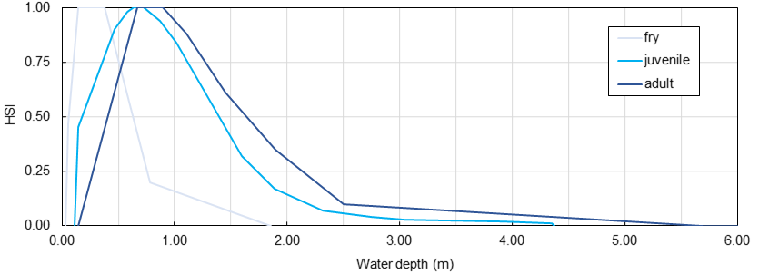
Figure 1:Habitat Suitability Index curves for the fry, juvenile, and adult life stages of rainbow trout in a cobble-bed river. Take care: HSI curves look different in any river and need to be established by an aquatic ecologist.
Das -Konzept berücksichtigt auch den sogenannten Cover-Habitat in Form des *cover Habitat Suitability Index * . Der Lebensraum Abdeckung ist das Ergebnis lokaler Turbulenzen, die durch Rauheitselemente wie Holz, Felsbrocken oder Brückenpfeiler verursacht werden. In dieser Übung werden wir uns jedoch nur mit hydraulischen Lebensraumeigenschaften befassen (ohne Lebensraum abzudecken).
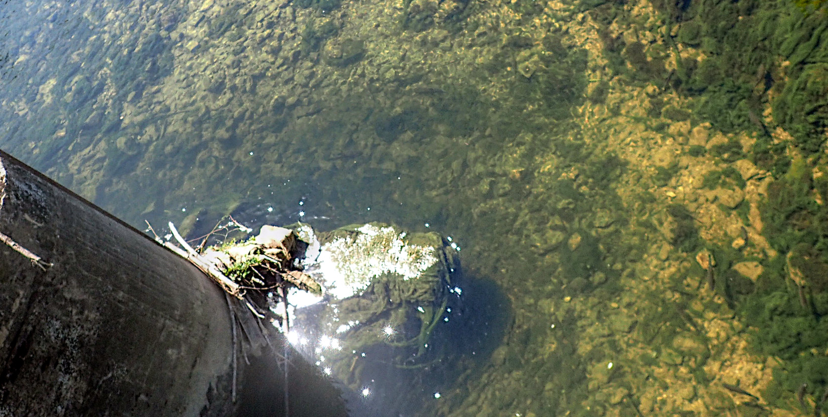
*Erwachsene Forellen schwimmen in einem Deckungsraum, der durch einen Brückensteg im oberen Neckar River geschaffen wurde. *
The combination of multiple values (e.g., water depth-related , flow velocity-related , grain size-related , and/or cover ) results in the combined Habitat Suitability Index . There are various calculation methods for combining different values into one value, where the geometric mean and the product are the most widely used deterministic combination methods:
Therefore, if the pixel-based values for water depth and flow velocity are known from a two-dimensional (2d) hydrodynamic model, then for each pixel the value can be calculated either as the product or geometric mean of the single-parameter rasters.
Dieses Habitat-Bewertungskonzept wurde von Bovee (1986) und Stalnaker et al. (1995) (direkter Download]) eingeführt. Diese Autoren bauten jedoch ihre nutzbare (physikalische) Habitatbewertung auf der Grundlage eindimensionaler (1d) numerischer Modelle auf, die im letzten Jahrtausend häufig verwendet wurden. Heute sind numerische 2D-Modelle auf dem neuesten Stand der Technik, um den physikalischen Lebensraum geospatially explizit basierend auf pixelbasierten -Werten zu bestimmen. Es gibt zwei verschiedene Optionen für die Berechnung der nutzbaren Lebensraumfläche () basierend auf pixelbasierten -Werten (und noch mehr Optionen finden Sie in der wissenschaftlichen Literatur).
Eine Alternative zur deterministischen Berechnung der - und -Werte eines Pixels ist ein unscharfer Logikansatz Noack et al., 2013. Beim Fuzzy-Logik-Ansatz werden Pixel beispielsweise als niedrig, mittel oder hohe Habitatqualität in Abhängigkeit von der zugehörigen Wassertiefe oder Strömungsgeschwindigkeit unter Verwendung kategorieller (niedrig, mittel oder hoch) Expertenbewertungs-basierter -Kurven klassifiziert. Der -Wert ergibt sich aus dem Schwerpunkt überlagerter Zugehörigkeitsfunktionen betrachteter Parameter (z. B. Wassertiefe und Strömungsgeschwindigkeit).
Nachhaltiges Flussmanagement beinhaltet die Herausforderung, einen aquatischen Lebensraum für Zielfischarten in verschiedenen Lebensphasen zu entwerfen. Das Konzept des nutzbaren physischen Lebensraums stellt ein leistungsfähiges Instrument dar, um die Bewertung der ökologischen Integrität von Flussmanagement- und Engineering-Maßnahmen zu nutzen. Durch die Berechnung der nutzbaren Lebensraumfläche vor und nach der Umsetzung von Maßnahmen lassen sich beispielsweise wertvolle Rückschlüsse auf die ökologische Integrität von Sanierungsbemühungen ziehen.
Diese Übung demonstriert die Verwendung von Ergebnissen der 2D-Hydrodynamik-Modellierung, um nutzbare Lebensräume algorithmisch zu bewerten, basierend auf der Berechnung geospatially expliziter -Werte.
Verfügbare Daten- und Codestruktur
Das folgende Flussdiagramm veranschaulicht den bereitgestellten Code und die Daten. Funktionen, Methoden und Dateien, die in dieser Übung erstellt werden sollen, werden in fett gedruckter, kursiver, GELBE-Schrift hervorgehoben.
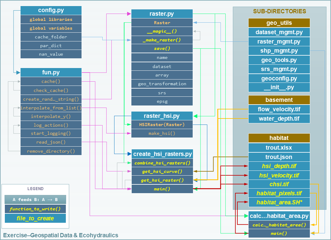
Figure 2:Struktur des bereitgestellten Template-Dateibaums und deren Beziehungen.
The provided QGIS project file visualize_with_QGIS.qgz helps to verify input raster datasets and results.
Zweidimensionale (2d) hydrodynamische Modellierung (Falter: BASEMENT)
This exercise uses (hydraulic) flow velocity and water depth rasters (GeoTIFFs) produced with the ETH Zurich*s BASEMENT software. Read more about hydrodynamic modeling with BASEMENT in the GRUNDLAGE chapter. The hydraulic rasters were produced with the BASEMENT developer’s example data from the Flaz River in Switzerland (read more on their website).
The water depth water_depth.tif and flow velocity flow_velocity.tif rasters are provided for this exercise in the folder /basement/.
Lebensfähigkeitsindex HSI-Kurven (folder: habitat)
Der /habitat/-Ordner im Übungs-Repository enthält -Kurven in Form einer xlsx-Arbeitsmappe (trout.xlsx) und in Form einer JSON-Datei (trout.json). Beide Dateien enthalten die gleichen Daten für die Regenbogenforelle eines hypothetischen Kopfsteinpflasterflusses und diese Übung verwendet nur die JSON-Datei (die Arbeitsmappe dient nur zur visuellen Verifizierung).
Code
HSI-Raster erstellen und kombinieren
Ergänzen Sie die __init__ Methode der RasterKlasse (raster.py)
The raster.py script imports the functions and libraries loaded in the fun.py script, and therefore, also the config.py script. For this reason, the NumPy and Pandas libraries are already available (as np and pd, respectively), and the geo_utils package is already imported as geo (import geo_utils as geo in config.py).
Die Raster-Klasse lädt jeden GeoTIFF-Dateinamen als georeferenziertes Array-Objekt, das mit mathematischen Operatoren verwendet werden kann. Zuerst werden wir die __init__-Methode durch ein Raster.name ergänzen (aus dem file_name-Argument entnehmen), sowie Georeferenzen und Array-Datensätze:
    # __init__(...) of Raster class in raster.py
        self.name = file_name.split("/")[-1].split("\\")[-1].split(".")[0]
Wenn das bereitgestellte file_name nicht existiert, erstellt die __init__-Methode ein neues Raster mit dem file_name (dieses Verhalten ist bereits in der if not os.path.exists(file_name)-Anweisung implementiert).
Als nächstes laden Sie osgeo.gdal.dataset, np.array und geo_transformation des Rasters. Verwenden Sie dazu das raster2array function aus diesem eBook, das auch im Paket geo utils der Übung (geo) implementiert ist:
    # __init__(...) of Raster class in raster.py
        self.dataset, self.array, self.geo_transformation = geo.raster2array(file_name, band_number=band)
To identify the EPSG number (Authority code) of a raster, retrieve the spatial reference system (SRS) of the raster. Also for this purpose we have already developed a function in the lecture with the get_srs from the theory section on reprojection. Load the SRS and the EPSG number using the get_srs function with the following two lines of code in the __init__ method:
    # __init__(...) of Raster class in raster.py
        self.srs = geo.get_srs(self.dataset)
        self.epsg = int(self.srs.GetAuthorityCode(None)
Die __init__-Methode der Raster-Klasse ist vollständig.
Vollständige magische Methoden der Raster Klasse (raster.py)
To enable mathematical operations between multiple instances of the Raster class, implement Überladen und magische Methoden that tell the class what to do when two Raster instances are for example added (+ sign), multiplied (* sign), or subtracted (- sign). For instance, implementing the magic methods __truediv__ (for using the / operator), __mul__ (for using the * operator), and __pow__ (for using the ** operator) will enable the usage of Raster instances like this:
# example for Raster instances, when operators are defined through magic methods

# load GeoTIFF rasters from file directory
velocity = Raster("/usr/geodata/u.tif")
depth = Raster("/usr/geodata/h.tif")

# calculate the Froude number using operators defined with magic methods
Froude = velocity / (depth * 9.81) ** 0.5

# save the new raster
Froude.save("/usr/geodata/froude.tif")
Die Klassenvorlage Raster enthält bereits eine beispielhafte Zaubermethode, um die Teilung zu ermöglichen (__truediv__):
    # Raster class in raster.py
    def __truediv__(self, constant_or_raster):
        try:
            self.array = np.divide(self.array, constant_or_raster.array)
        except AttributeError:
            self.array /= constant_or_raster
        return self._make_raster("div")
Here is what the __truediv__ method does:
The input argument
constant_or_rastercan be anotherRasterinstance that has anarrayattribute or a numeric constant (e.g., 9.81).The method tries to invoke the array attribute of
constant_or_raster.If
constant_or_rasteris a raster object, then invokingcontant_or_raster.arrayis successful. In this caseself.arrayis overwritten with the element-wise division of the array bycontant_or_raster.array. The element-wise division builds on NumPys built-in function np.divide, which is a computationally efficient wrapper of C/C++ code (much faster than a Python loop over array elements).If
constant_or_rasteris a numeric value, then invokingcontant_or_raster.arrayresults in anAttributeErrorand the__truediv__method falls in theexcept AttributeErrorstatement, whereself.arrayis simply divided byconstant_or_raster.
Die Methode gibt das Ergebnis der Pseudo-Private-Methode
self._make_raster("div")zurück ([recall PEP 8 Code-Stil und Konventionen, was einer neuenRaster-Instanz der tatsächlichenRaster-Instanz geteilt durchconstant_or_rasterentspricht). Die neueRaster-Instanz ist eine temporäre GeoTIFF-Datei im Cache-Ordner (rufen Sie die cache function zurück). So sieht die pseudo-private Methode_make_raster(self, file_marker)aus:
Diese Funktion:
Verwendet das Argument string-Typ
file_marker, um es dem Dateinamen der Basis GeoTIFF zusammen mit einem zufälligen, vier Zeichen langen string hinzuzufügen (rufen Sie das create_random_string zurück).file_markerist für jeden implementierten Operator einzigartig. Für die__truediv__Methode verwenden Siefile_marker="div". Daher ist der temporäre GeoTIFF-Dateiname alscache_folder + self.name + f_endingdefiniert (z. B."C:\Excercise-geco\__cache__\velocity__divhjev__.tif").Wendet die Funktion Erstellen Sie einen Raster (Raster-Array) von
geo_utilsan, um das temporäre GeoTIFF in den__cache__-Ordner mit dem räumlichen Referenzsystem des ursprünglichen Rasters zu schreiben.returns eine neueRasterInstanz der temporären, zwischengespeicherten GeoTIFF Datei.
If you find the _make_raster method confusing...
Then you have a point. The above-described approach implements the _make_raster method to reuse the temporary GeoTIFFs later with both constants (float) and arrays, but there is a more elegant way to return a new Raster instance. However, returning a new instance of the same class requires that the input argument must be an instance of the class itself (i.e., Raster) and not a numeric variable. The alternative solution for returning a Raster instance starts with a different implementation of the magic method (e.g., __truediv__) and requires importing Python4-style annotations. Therefore, the first line of the script must include (only works with Python 3.7 and higher) the following import:
from __future__ import annotationsThen rewrite the __truediv__ method:
    def __truediv__(self, other: Raster) -> Raster:
        f_ending = "__div%s__.tif" % create_random_string(4)
        return Raster(file_name=cache_folder + self.name + f_ending,
                      raster_array=np.divide(self.array, other.array),
                      epsg=self.epsg,
                      geo_info=self.geo_transformation)
In diesem Fall ist die _make_raster-Methode veraltet. Lesen Sie mehr über das Zurückgeben von Instanzen derselben Klasse auf Stack overflow].
Wenn Sie die _make_raster-Methode verwenden, fügen Sie die folgenden magischen Methoden zur Raster-Klasse hinzu (Funktionsplatzhalter sind bereits in der raster.py-Vorlage vorhanden):
__add__(+Operator):
        try:
            self.array += constant_or_raster.array
        except AttributeError:
            self.array += constant_or_raster
return self._make_raster("add")__mul__(*Operator):
        try:
            self.array = np.multiply(self.array, constant_or_raster.array)
        except AttributeError:
            self.array *= constant_or_raster
return self._make_raster("mul")__pow__(**Operator):
        try:
            self.array = np.power(self.array, constant_or_raster.array)
        except AttributeError:
            self.array **= constant_or_raster
return self._make_raster("pow")__sub__(-Operator):
        try:
            self.array -= constant_or_raster.array
        except AttributeError:
            self.array -= constant_or_raster
        return self._make_raster("sub")
Das letzte Element, das in der Raster-Klasse abgeschlossen werden muss, ist die eingebaute save-Methode, die ein file_name (string)-Argument erhält, das das Verzeichnis und den Save-as-Namen der Raster-Instanz definiert:
        save_status = geo.create_raster(file_name, self.array, epsg=self.epsg, nan_val=0.0, geo_info=self.geo_transformation)
        return save_status
Warum brauchen wir die save_status-Variable? Erstens gibt es an, ob das Speichern des Rasters erfolgreich war (save_status=0), und zweitens könnten diese Informationen verwendet werden, um das Raster aus dem __cache__-Ordner zu löschen und den Speicher zu spülen (fühlen Sie sich frei, dies zu tun, um den Code zu beschleunigen).
Schreiben Sie HSI und cHSI-Raster-Erstellungsskript
Das bereitgestellte create_hsi_rasters.py Skript enthält bereits die erforderlichen Paketimporte, eine if __name__ == '__main__' stand-alone-Anweisung sowie die void main, get_hsi_curve, get_hsi_raster und combine_hsi_rasters Funktionen:
Die if __name__ == '__main__'-Anweisung enthält einen Zeitzähler (perf_counter), der anzeigt, wie lange das Skript dauert (normalerweise zwischen 3 und 6 Sekunden). Stellen Sie sicher, dass
Die
parameters-Liste enthält"velocity"und"depth"(gemäßpar_dictimconfig.py-Skript),die Dateipfade korrekt definiert sind und
Eine Lebensphase wird definiert (d.h. entweder
"fry","juvenile","adult"oder"spawning"gemäß der /habitat/fish.xlsx Arbeitsmappe).
The following paragraphs show step by step how to load the curves from the JSON file (get_hsi_curve), apply them to the flow_velocity and water_depth rasters (get_hsi_raster), and combine the resulting rasters into rasters (combine_hsi_rasters).
The get_hsi_curve function will load the curve from the JSON file (/habitat/trout.json) in a dictionary for the two parameters "velocity" and "depth". Thus, the goal is to create a curve_data dictionary that contains one Pandas DataFrame object for all parameters (i.e., velocity and depth). For example, curve_data["velocity"]["u"] will be a Pandas Series of velocity entries (in m/s) that corresponds to curve_data["velocity"]["HSI"], which is a Pandas Series of values. Similarly, curve_data["depth"]["h"] is a Pandas Series of depth entries (in meters) that corresponds to curve_data["depth"]["HSI"], which is a Pandas Series of values (corresponds to the curves shown in the HSI graphs above). To extract the desired information from the JSON file, get_hsi_curve takes three arguments (json_file, life_stage, and parameters) in order to:
Get the information stored in the JSON file with the
read_jsonfunction (see above).Instantiate a void
curve_dataWörterbuch that will contain the PandasDataFrames for"velocity"and"depth".Führen Sie eine Schleife über die (zwei) Parameter (
"velocity"und"depth"), in denen es:Creates a void
par_pairsListe for storing pairs of parameter (par) - values as nested lists.Iterates through the length of provided curve data, where valid data pairs (e.g.,
[u_value, HSI_value]) are appended to thepar_pairsListe. This iteration is what actually creates the nested Liste.Converts the final
par_pairslist to a PandasDataFramethat it adds to thecurve_dataWörterbuch.
returnthecurve_dataWörterbuch with its PandasDataFrames.
# create_hsi_rasters.py
def get_hsi_curve(json_file, life_stage, parameters):
    # read the JSON file with fun.read_json
    file_info = read_json(json_file)
    # instantiate output dictionary
    curve_data = {}
    # iterate through parameter list (e.g., ["velocity", "depth"])
    for par in parameters:
        # create a void list to store pairs of parameter-HSI values as nested lists
        par_pairs = []
        # iterate through the length of parameter-HSI curves in the JSON file
        for i in range(0, file_info[par][life_stage].__len__():
            # if the parameter is not empty (i.e., __len__ > 0), append the parameter-HSI (e.g., [u_value, HSI_value]) pair as nested list
            if str(file_info[par][life_stage][i]["HSI"]).__len__() > 0:
                try:
                    # only append data pairs if both parameter and HSI are numeric (floats)
                    par_pairs.append([float(file_info[par][life_stage][i][par_dict[par]]),
                                      float(file_info[par][life_stage][i]["HSI"])])
                except ValueError:
                    logging.warning("Invalid HSI curve entry for {0} in parameter {1}.".format(life_stage, par)
        # add the nested parameter pair list as pandas DataFrame to the curve_data dictionary
        curve_data.update({par: pd.DataFrame(par_pairs, columns=[par_dict[par], "HSI"])})
    return curve_data
In the main function, call get_hsi_curves to get the curves as a Wörterbuch. In addition, implement the cache and the log_actions wrappers (recall the descriptions of provided functions) for the main function:
# create_hsi_rasters.py

...

@log_actions
@cache
def main():
    # get HSI curves as pandas DataFrames nested in a dictionary
    hsi_curve = get_hsi_curve(fish_file, life_stage=life_stage, parameters=parameters)

...
With the provided HSIRaster (raster_hsi.py) class, the rasters can be conveniently created in the get_hsi_raster function. Before using the HSIRaster class, make sure to understand how it works. The HSIRaster class inherits from the Raster class and initiates its parent class in its __init__ method through Raster.__init__(self, file_name=file_name, band=band, raster_array=raster_array, geo_info=geo_info). Then, the class calls its make_hsi method, which takes an curve (nested Liste) of two equal Liste pairs (Liste of parameters and Liste of values) as argument. The make_hsi method:
Extracts parameter values (e.g., depth or velocity) from the first element of the nested
hsi_curvesListe, and values from the second element of the nestedhsi_curvesListe.Uses NumPys built-in
np.nditerfunction, which iterates through NumPy arrays with high computational efficiency (read more aboutnditer).The
nditerloop passes thepar_valuesasx_valuesListe argument and thehsi_valuesasy_valuesListe arguments to theinterpolate_from_listfunction (recall the function descriptions above).The array values (i.e., flow velocity or water depth) correspond to the
xi_valuesListe argument of theinterpolate_from_listfunction.The
interpolate_from_listfunction then identifies for each element of thexi_valuesListe the closest elements ( values) in thex_valuesListe and the corresponding positions in they_valuesListe.Die Funktion
interpolate_from_listübergibt die identifizierten Werte an die Funktioninterpolate_y, die dann den entsprechendenyi-Wert linear interpoliert (d.h. einen -Wert).Thus, the flow velocity or water depths in
self.arrayare row-wise (row-by-row) replaced by values.
returns eineRaster-Instanz mit der pseudo-privaten_make_raster-Methode (recall its contents).
# raster_hsi.py
from raster import *

class HSIRaster(Raster):
    def __init__(self, file_name, hsi_curve, band=1, raster_array=None, geo_info=False):
        Raster.__init__(self, file_name=file_name, band=band, raster_array=raster_array, geo_info=geo_info)
        self.make_hsi(hsi_curve)

    def make_hsi(self, hsi_curve):
        par_values = hsi_curve[0]
        hsi_values = hsi_curve[1]
        try:
            with np.nditer(self.array, flags=["external_loop"], op_flags=["readwrite"]) as it:
                for x in it:
                    x[...] = interpolate_from_list(par_values, hsi_values, x)
        except AttributeError:
            print("WARNING: np.array is one-dimensional.")
        return self._make_raster("hsi")
Ändern Sie die Funktion get_hsi_rasters, um ein HSIRaster-Objekt direkt zurückzugeben:
# create_hsi_rasters.py

...

def get_hsi_raster(tif_dir, hsi_curve):
    return HSIRaster(tif_dir, hsi_curve)
...
The get_hsi_raster function requires two arguments, which it must receive from the main function. For this reason, iterate over the parameters Liste in the main function and extract the corresponding raster directories from the tifs Wörterbuch (recall the variable definition in the standalone statement). In addition, save the Raster objects returned by the get_hsi_raster function in another Wörterbuch (eco_rasters) to combine them in the next step into a raster.
# create_hsi_rasters.py

...

@log_actions
@cache
def main():
    # get HSI curves as pandas DataFrames nested in a dictionary
    hsi_curve = get_hsi_curve(fish_file, life_stage=life_stage, parameters=parameters)

        # create HSI rasters for all parameters considered and store the Raster objects in a dictionary
    eco_rasters = {}
    for par in parameters:
        hsi_par_curve = [list(hsi_curve[par][par_dict[par]]),
                         list(hsi_curve[par]["HSI"])]
        eco_rasters.update({par: get_hsi_raster(tif_dir=tifs[par], hsi_curve=hsi_par_curve)})
        eco_rasters[par].save(hsi_output_dir + "hsi_%s.tif" % par)
...
Natürlich kann man die Parameter Liste auch direkt in der Funktion get_hsi_raster durchschleifen.
Next, we come to the reason why we had to define magic methods for the Raster class: combine the rasters using both combination formulae presented above (recall the product and geometric mean formulae), where "geometric_mean" should be used by default. The combine_hsi_rasters function accepts two arguments (a Liste of Raster objects corresponding to rasters and the method to use as string).
If the method corresponds to the default value "geometric_mean", then the power to be applied to the product of the Raster Liste is calculated from the nth root, where n corresponds to the number of Raster objects in the raster_list. Otherwise (e.g., method="product"), the power is exactly 1.0.
The combine_hsi_rasters function initially creates an empty Raster in the cache_folder, with each cell having the value 1.0 (filled through np.ones). In a loop over the Raster elements of the raster_list, the function multiplies each raster with the raster.
Finally, the function returns the product of all rasters to the power of the previously determined power value.
# create_hsi_rasters.py
def combine_hsi_rasters(raster_list, method="geometric_mean"):
    if method is "geometric_mean":
        power = 1.0 / float(raster_list.__len__()
    else:
        # supposedly method is "product"
        power = 1.0

    chsi_raster = Raster(cache_folder + "chsi_start.tif",
                         raster_array=np.ones(raster_list[0].array.shape),
                         epsg=raster_list[0].epsg,
                         geo_info=raster_list[0].geo_transformation)
    for ras in raster_list:
        chsi_raster = chsi_raster * ras

    return chsi_raster ** power
Um das create_hsi_rasters.py-Skript abzuschließen, implementieren Sie den Aufruf der combine_hsi_rasters-Funktion in der main-Funktion und speichern Sie das Ergebnis als GeoTIFF-Raster im /habitat/-Ordner:
# create_hsi_rasters.py

...

@log_actions
@cache
def main():
    ...

    for par in parameters:
        hsi_par_curve = [list(hsi_curve[par][par_dict[par]]),
                         list(hsi_curve[par]["HSI"])]
        eco_rasters.update({par: get_hsi_raster(tif_dir=tifs[par], hsi_curve=hsi_par_curve)})
        eco_rasters[par].save(hsi_output_dir + "hsi_%s.tif" % par)

    # get and save chsi raster
    chsi_raster = combine_hsi_rasters(raster_list=list(eco_rasters.values(),
                                      method="geometric_mean")
    chsi_raster.save(hsi_output_dir + "chsi.tif")
...
Führen Sie den HSI- und cHSI-Code aus
Ein erfolgreicher Ablauf des Skripts create_hsi_rasters.py sollte so aussehen (in PyCharm):
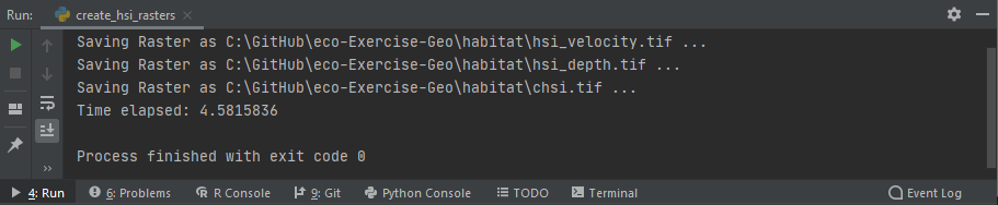
Figure 3:Eine Windows Python-Konsole, auf der die oben erstellten Skripte ausgeführt werden.
Plotted in QGIS, the GeoTIFF raster should look like this:
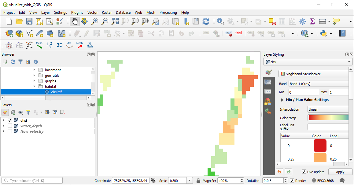
Figure 4:Das cHSI-Raster in QGIS aufgetragen, wo schlechte physikalische Habitatqualität (cHSI nahe 0,0) in rot und hohe physikalische Habitatqualität (cHSI nahe 1,0) in grün gefärbt ist.
Ergebnisinterpretation
The presentation of the raster shows that preferred habitat areas for juvenile trout exist only close to the banks. Also, numerical artifacts of the triangular mesh used by GRUNDLAGE are visible. Therefore, the question arises whether the calculated flow velocities and water depths, and in consequence also the values, close to the banks can be considered representative.
Berechnen nutzbarer Lebensraum UHA
Schreiben Sie den Code
The rasters enable the calculation of the available usable habitat area. The previous section featured examples using the fish species trout and its juvenile life stage, for which we will determine here the usable habitat area (in m) using a threshold value (rather than the pixel area weighting approach). So we follow the threshold formula described above, using a threshold value of . Thus, every pixel that has a value of 0.4 or greater counts as usable habitat area.
Aus technischer Sicht geht es in diesem Teil der Übung darum, ein Raster in ein Polygon-Shapefile umzuwandeln sowie auf die *Attributtabelle * der Shapefile zuzugreifen und zu modifizieren.
Ähnlich wie bei der Erstellung des -Rasters gibt es für diesen Teil der Übung ein Vorlagenskript namens calculate_habitat_area.py, das Paket- und Modulimporte, eine if __name__ == '__main__'-Stand-alone-Anweisung sowie die void main und calculate_habitat_area-Funktionen enthält. (uha-templat) =
Das Template-Skript sieht so aus:
# this is calculate_habitat_area.py (template)
from fun import *
from raster import Raster


def calculate_habitat_area(layer, epsg):
    pass


def main():
    pass


if __name__ == '__main__':
    chsi_raster_name = os.path.abspath("") + "\\habitat\\chsi.tif"
    chsi_threshold = 0.4

    main()
Stellen Sie in der if __name__ == '__main__'-Anweisung sicher, dass die globale Variable chsi_raster_name dem Verzeichnis des -Rasters entspricht, das im vorherigen Abschnitt erstellt wurde. Die andere globale Variable (chsi_threshold) entspricht dem -Wert von 0,4, den wir zusammen mit threshold formula verwenden werden.
In the main function, start with loading the raster (chsi_raster) as a Raster object. Then, access the NumPy array of the raster and compare it with chsi_threshold using NumPys built-in greater_equal function. np.greater_equal takes an array as first argument and a second argument, which is the condition that can be a numeric variable or another NumPy array. Then, np.greater_equal checks if the elements of the first array are greater than or equal to the second argument. In the case of the second argument being an array, this is an element-wise comparison. The result of np.greater_equal is a Boolean array (True where the greater-or-equal condition is fulfilled and False otherwise). However, to create an osgeo.gdal.Dataset object from the result of np.greater_equal, we need a numeric array. For this reason, multiply the result of np.greater_equal by 1.0 and assign it as a new NumPy array of zeros (False) and ones (True) to a variable named habitat_pixels (see the code block below).
Erstellen Sie mit dem habitat_pixels-Array und der Georeferenz von chsi_raster ein neues integerGeoTIFF-Raster mit der Funktion create raster (auch in flusstools.geotools] verfügbar); verwenden Sie hier geo.create_raster. Im folgenden Codeblock wird das neue Raster im /habitat/-Ordner der Übung als habitat-pixels.tif gespeichert.
# calculate_habitat_area.py
...

def main():
    # open the chsi raster
    chsi_raster = Raster(chsi_ras_name)
    # extract pixels where the physical habitat quality is higher than the user threshold value
    habitat_pixels = np.greater_equal(chsi_raster.array, chsi_threshold_value) * 1
    # write the habitat pixels to a binary array (0 -> no habitat, 1 -> usable habitat)
    geo.create_raster(os.path.abspath("") + "\\habitat\\habitat-pixels.tif",
                      raster_array=habitat_pixels,
                      epsg=chsi_raster.epsg,
                      geo_info=chsi_raster.geo_transformation)
...
In the next step, convert the habitat pixel raster into a polygon shapefile and save it in the /habitat/ folder as habitat-area.shp. The conversion of a raster into a polygon shapefile requires that the raster contains only integer values, which is the case in the habitat pixel raster (only zeros and ones - recall Raster zu Polygon). Use the raster2polygon function in the geo_utils folder (package) to create the new polygon shapefile, specify habitat-pixels.tif as raster_file_name to be converted, and /habitat/habitat-area.shp as output file name. The geo.raster2polygon function returns an osgeo.ogr.DataSource object and we can pass its layer including the information of the EPSG authority code (from chsi_raster) directly to the not-yet-written calculate_habitat_area() function:
# calculate_habitat_area.py
...

def main():
    ... (create habitat pixels raster)

    # convert the raster with usable pixels to polygon (must be an integer raster!)
    tar_shp_file_name = os.path.abspath("") + "\\habitat\\habitat-area.shp"
    habitat_polygons = geo.raster2polygon(os.path.abspath("") + "\\habitat\\habitat-pixels.tif",
                                          tar_shp_file_name)

    # calculate the habitat area (will be written to the attribute table)
    calculate_habitat_area(habitat_polygons.GetLayer(), chsi_raster.epsg)
...
For the calculate_habitat_area() function to produce what its name promises, we need to populate this function as well. For this purpose, use the epsg integer argument to identify the unit system of the shapefile.
# calculate_habitat_area.py
...

def calculate_habitat_area(layer, epsg):
    # retrieve units
    srs = geo.osr.SpatialReference()
    srs.ImportFromEPSG(epsg)
    area_unit = "square %s" % str(srs.GetLinearUnitsName()
...To determine the habitat area, the area of each polygon must be calculated. For this purpose, add a new field to the layer in the Attribute Table, name it "area", and assign a geo.ogr.OFTReal (numeric) data type (recall how to create a field an data types).
Then, create a void Liste called poly_size, in which we will write the area of all polygons that have a field value of 1. To access the individual polygons (features) of the layer, iterate through all features using a for loop, which:
Extracts the polygon of every
featureusingpolygon = feature.GetGeometryRef()Appends the polygon’s area size to the
poly_sizeListe if the field"value"of thepolygon(at position 0:feature.GetField(0)) is 1 (True).Writes the polygon’s area size to the Attribute Table with
feature.SetField("area", polygon.GetArea().Speichert die Änderungen (berechneter Bereich) in der Shapefile
layermitlayer.SetFeature(feature).
The last information needed after the for loop is the total area of the "value"=1 polygons, which we get by writing the sum of the poly_size Liste to the console. Therefore, the second and last part of the calculate_habitat_area function looks like this:
# calculate_habitat_area.py
...
def calculate_habitat_area(layer, epsg):

    ... (extract unit system information)

    # add area field
    layer.CreateField(geo.ogr.FieldDefn("area", geo.ogr.OFTReal)

    # create list to store polygon sizes
    poly_size = []

    # iterate through geometries (polygon features) of the layer
    for feature in layer:
        # retrieve polygon geometry
        polygon = feature.GetGeometryRef()
        # add polygon size if field "value" is one (determined by chsi_treshold)
        if int(feature.GetField(0):
            poly_size.append(polygon.GetArea()
        # write area to area field
        feature.SetField("area", polygon.GetArea()
        # add the feature modifications to the layer
        layer.SetFeature(feature)

    # calculate and print habitat area
    print("The total habitat area is {0} {1}.".format(str(sum(poly_size), area_unit)

...Führen Sie den nutzbaren Lebensraum-Berechnungscode aus
Ein erfolgreicher Ablauf des Skripts calculate_habitat_area.py sollte so aussehen (in PyCharm):
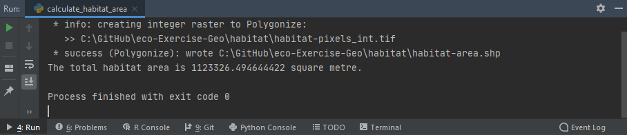
Figure 5:Erfolgreicher Ablauf des Skripts calculate habitat area.py.
Aufgetragen in QGIS, sieht das habitat-area Shapefile so aus (verwende Categorized Symbologie):
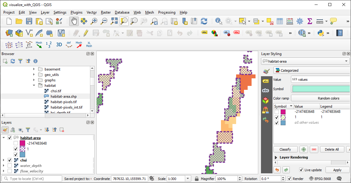
Figure 6:The habitat-area shapefile plotted in QGIS with Categorized symbology, where the usable habitat area ( 0.4) is delineated by the hatched purple patches and their dashed outlines.
Ergebnisinterpretation
The of the analyzed river section represents a very small share of the total wetted area, which can be interpreted as an ecologically poor status of the river. However, a glance at a map and the simulation files of the Flaz example of BASEMENT suggests that at a discharge of 50 m/s, a flood situation can be assumed. As during floods, there are generally higher flow velocities, which are out-of-favor of juvenile fish, the small usable habitat area is finally not surprising.
- Noack, M., Schneider, M., & Wieprecht, S. (2013). Ecohydraulics: an integrated approach (I. Maddock, A. Harby, P. Kemp, & P. Wood, Eds.; pp. 75–91). Wiley-Blackwell. 10.1002/9781118526576
- Bovee, K. D. (1986). Development and evaluation of Habitat Suitability Criteria for use in the instream flow incremental methodology (Techreport No. 21). National Ecology Center, U.S. Fish. https://pubs.er.usgs.gov/publication/70121265
- Stalnaker, C., Lamb, B. L., Henriksen, J., Bovee, K., & Bartholow, J. (1995). The Instream Flow Incremental Methodology - A Primer for IFIM. National Biological Service, U.S. Department of the Interior, Opler, Paul A. www.dtic.mil/cgi-bin/GetTRDoc?AD=ADA322762
- Yao, W., Bui, M. D., & Rutschmann, P. (2018). Development of eco-hydraulic model for assessing fish habitat and population status in freshwater ecosystems. Ecohydrology, 11(5), 1–17. 10.1002/eco.1961
- Tuhtan, J. A., Noack, M., & Wieprecht, S. (2012). Estimating stranding risk due to hydropeaking for juvenile European grayling considering river morphology. KSCE Journal of Civil Engineering, 16(2), 197–206. 10.1007/s12205-012-0002-5