This section introduces geospatial analysis of raster (gridded) data with gdal and rasterstats. For interactive reading and executing code blocks  , or install Python and JupyterLab locally.
Watch this section and the Python tutorials in video formats
Watch this section as a video on the @Hydro-Morphodynamics channel on YouTube.
Belastungsraster
vorhandene Rasterdaten öffnen
Raster data can be opened in Python code as an instance of gdal.Open("FILENAME"). The following code block provides a function to open any raster specified with the file_name input argument. One of the most important elements when dealing with raster data is the raster band, which takes on a similar data carrier role as GetLayer in shapefile handling. To access the raster band, the below-shown open_raster function:
Enables error and warning feedback with
gdal.UseExceptions()(this step is vital when using gdal).Opens the provided raster
file_nameembraced bytry-exceptstatements to inform if and why a potential error occurred while opening the raster.Opens the raster band number stated in the optional
band_numberkeyword argument withraster_band = raster.GetRasterBand(band_number)(the default value is1).Gibt die Objekte Raster und Rasterband zurück.
Run this notebook with marimo
Dieses Notizbuch ist auch als marimoNotebook (ein reaktives Python-Notizbuch, das als reine .py-Datei gespeichert ist) im marimo
Repository:
git clone https://github.com/sschwindt/marimo-python-course.gitDie Kursumgebung erstellen und aktivieren:
conda env create -f environment.ymlundconda activate hy-marimoStarten Sie im Ordner Repository das Notebook mit
marimo edit geo02-raster.py
from osgeo import gdal
import numpy as np


def open_raster(file_name, band_number=1):
    """
    Open a raster file and access its bands
    :param file_name: STR of a raster file directory and name
    :param band_number: INT of the raster band number to open (default: 1)
    :output: osgeo.gdal.Dataset, osgeo.gdal.Band objects
    """
    gdal.UseExceptions()
    # open raster file or return None if not accessible
    try:
        raster = gdal.Open(file_name)
    except RuntimeError as e:
        print("ERROR: Cannot open raster.")
        print(e)
        return None
    # open raster band or return None if corrupted
    try:
        raster_band = raster.GetRasterBand(band_number)
    except RuntimeError as e:
        print("ERROR: Cannot access raster band.")
        print(e)
        return None
return raster, raster_bandTo use the open_raster function, call it with a file name as shown in the following code block with the h001000.tif raster from the River Architect sample data. The script immediately closes the raster again by overwriting the variable with a None-instance to avoid the GeoTIFF file being locked afterward.
import os
file_name = r"" + os.getcwd() + "/geodata/rasters/h001000.tif"
src, depth = open_raster(file_name)
print(src)
print(depth)
depth = None
<osgeo.gdal.Dataset; proxy of <Swig Object of type 'GDALDatasetShadow *' at 0x77015c0a7b70> >
<osgeo.gdal.Band; proxy of <Swig Object of type 'GDALRasterBandShadow *' at 0x77015c0f39b0> >
Rasterband Statistiken und Toolbox-Skripte
Once the raster and its band are loaded with the above open_raster function, we can access statistical information (e.g., the minimum or the maximum), identify the no-data value (i.e., a pre-defined value that is assigned to pixels without value), or the type of units used.
Python-Skripte zur Verarbeitung von Geodaten können auch als Plugins in GIS-Desktop-Anwendungen eingebettet werden (z.B. als Plugins in QGIS oder Toolbox in ArcGIS Pro). Um ein Python-Skript in einer GIS-Desktopanwendung auszuführen, sollte es als eigenständiges Skript geschrieben werden, das Eingabeargumente empfangen kann. Der interessierte Leser kann mehr über die Implementierung von Plugins in QGIS in der QGIS docs] erfahren.
Here we will only write the next code block so that it can be run in a console/terminal application as a standalone script (recall the instructions for writing standalone script).
import sys
from osgeo import gdal

# make sure to use exceptions
gdal.UseExceptions()

def how2use():
    # provide usage instructions for the script
    print("""
    $ raster_band_info.py [ band number ] input-raster
    """)
    # exit program if wrong input arguments provided
    sys.exit(1)


def get_color_bands(raster_band):
    """
    :param raster_band: osgeo.gdal.Band object
    :output: list of color bands used in raster_band
    """

    # get ColorTable and return False if None
    color_table = raster_band.GetColorTable()
    if color_table is None:
        print("Band has no ColorTable.")
        return None
    else:
        print("Found %i color definitions." % int(color_table.GetCount()))

    # iterate through color_table and append objects found to colors_bands list
    color_bands = []
    for c in range(0, color_table.GetCount() ):
        entry = color_table.GetColorEntry(c)
        if not entry:
            continue
        color_bands.append(str(color_table.GetColorEntryAsRGB(c, entry)))
    return color_bands

def main(band_number, input_file):
    src, band = open_raster(input_file)
    print("Band minimum: ", band.GetMinimum())
    print("Band maximum: ", band.GetMaximum())
    print("No-data value: ", band.GetNoDataValue())
    print("Band unit type: ", band.GetUnitType())

    try:
        print(", ".join(get_color_bands(band)))
    except TypeError:
        print("ColorTable: None")

if __name__ == '__main__':
    # make standalone
    if len( sys.argv ) < 3:
        print("""
        ERROR: Provide two arguments:
        1) the band number (int) and 2) input raster directory (str)
        """)
        how2use()

    main(int(sys.argv[1]), str(sys.argv[2]))
To run this script, save it as raster_band_info.py (e.g., in C:\temp in Windows or ~/temp/ in Linux) and navigate to the script directory in a terminal interface (e.g., in PyCharm’s Terminal, Anaconda Prompt, or the Linux Terminal) using the cd command. Then run the script to get statistics of the water depth raster h001000.tif with (in Windows):
C:\temp\ python raster_band_info.py 1 "C:\temp\geodata\rasters\h001000.tif"On Linux and with the flussenv activated, for example:
python raster_band_info.py 1 "~/temp/geodata/rasters/h001000.tif"Band minimum: 0.0
Band maximum: 7.0613012313843
No-data value: -3.4028234663852886e+38
Band unit type:
Band has no ColorTable.
ColorTable: NoneErstellen und Speichern eines Rasters (aus Array)
Rastertreiber
Just like for shapefile files, the appropriate gdal driver (analogous to ogr drivers) must be loaded to save a raster. To get a full list of gdal raster drivers run:
driver_list = [str(gdal.GetDriver(i).GetDescription()) for i in range(gdal.GetDriverCount())]
driver_list.sort()
print(", ".join(driver_list[:]))
AAIGrid, ACE2, ADRG, AIG, AIVector, AVCBin, AVCE00, AirSAR, AmigoCloud, BIGGIF, BMP, BSB, BT, BYN, CAD, CALS, CEOS, COASP, COG, COSAR, CPG, CSV, CSW, CTG, Carto, DAAS, DERIVED, DGN, DIMAP, DOQ1, DOQ2, DTED, DXF, ECRGTOC, EDIGEO, EEDA, EEDAI, EHdr, EIR, ENVI, ERS, ESAT, ESRI Shapefile, ESRIC, ESRIJSON, Elasticsearch, FAST, FlatGeobuf, GDALG, GFF, GIF, GML, GMLAS, GNMDatabase, GNMFile, GPKG, GPSBabel, GPX, GRASSASCIIGrid, GS7BG, GSAG, GSBG, GSC, GTFS, GTI, GTX, GTiff, GXF, GenBin, GeoJSON, GeoJSONSeq, GeoRSS, HF2, HFA, HTTP, ILWIS, IRIS, ISCE, ISG, ISIS2, ISIS3, Idrisi, Interlis 1, Interlis 2, JAXAPALSAR, JDEM, JML, JPEG, JPEGXL, JSONFG, KML, KMLSUPEROVERLAY, KRO, L1B, LAN, LCP, LIBERTIFF, LIBKML, LOSLAS, LVBAG, Leveller, MAP, MBTiles, MEM, MFF, MFF2, MRF, MSGN, MVT, MapInfo File, MapML, MiraMonRaster, MiraMonVector, NAS, NDF, NGSGEOID, NGW, NITF, NOAA_B, NSIDCbin, NTv2, NUMPY, NWT_GRC, NWT_GRD, OAPIF, ODS, OGCAPI, OGR_GMT, OGR_PDS, OGR_VRT, OSM, OpenFileGDB, PAux, PCIDSK, PCRaster, PDS, PDS4, PGDUMP, PLMOSAIC, PLSCENES, PMTiles, PNG, PNM, PRF, RCM, RIK, RMF, ROI_PAC, RPFTOC, RRASTER, RS2, RST, S57, SAFE, SAGA, SAR_CEOS, SENTINEL2, SIGDEM, SNAP_TIFF, SNODAS, SQLite, SRP, SRTMHGT, STACIT, STACTA, SXF, Selafin, TGA, TIL, TSX, Terragen, TopoJSON, USGSDEM, VDV, VFK, VICAR, VRT, WAsP, WCS, WEBP, WFS, WMS, WMTS, XLSX, XYZ, ZMap, Zarr
Rasterdatentypen
Die Ausgangs-Rasterpixel können einer der folgenden Datentypen sein (Quelle: gdal.org/doxygen/]):
GDT_UnknownUnbekannter oder unspezifizierter TypGDT_Byte8 Bit unsignierte GanzzahlGDT_UInt1616 Bit unsignierte GanzzahlGDT_Int1616 bit signiert ganzzahligGDT_UInt3232 Bit unsignierte GanzzahlGDT_Int3232 bit signiert ganzzahligGDT_Float3232 Bit Floating PointGDT_Float6464 Bit Floating PointGDT_CInt16Complex Int16GDT_CInt32Complex Int32GDT_CFloat32Complex Float32GDT_CFloat64Complex Float64
Erstellen Sie einen Raster (Raster-Array)
Knowing the basics of raster handling, data types, and Python, we can create a raster from a numeric array. Since a raster is basically a georeferenced array, it is convenient to convert a numpy array into a raster (band). The function blocks feature the conversion of a numpy array into a GeoTIFF raster according to the following workflow:
Schauen Sie sich den GeoTIFF-Treiber an (
driver = gdal.GetDriverByName('GTiff')).Retrieve the array size and (number of rows
rowsand columnscols).Erstellen Sie ein neues GeoTIFF-Raster (
new_raster = driver.Create(file_name, cols, rows, 1, eType=rdtype)), in demfile_nameist das Verzeichnis und der Name der neuen Rasterdatei, die auf.tifendet (z. B."C:\\temp\\rasters\\new.tif").cols,rowsrepräsentieren die Array-Form undeTypeist der Geodatentyp (siehe oben).
Legen Sie den geografischen Ursprung fest, der im Parameter
origin(tuple) gespeichert ist, und definieren Sie diepixel_widthundpixel_height(Pixeleinheiten, die mitsrsdefiniert sind - siehe unten).Replace
np.nanvalues in the numpy array withnan_value.Instantiate a
bandobject, set theNoDataValuetonan_value, and write the array to theband.Erstellen Sie ein räumliches Referenzsystemobjekt (
srs) als Funktion des Eingangsparametersepsgund exportieren Sie es in das WKT-Format.Geben Sie das Raster frei (aus dem Cache fließen).
from osgeo import osr


def create_raster(file_name, raster_array, origin=None, epsg=4326, pixel_width=10, pixel_height=10,
                  nan_value=-9999.0, rdtype=gdal.GDT_Float32, geo_info=False):
    """
    Convert a numpy.array to a GeoTIFF raster with the following parameters
    :param file_name: STR of target file name, including directory; must end on ".tif"
    :param raster_array: np.array of values to rasterize
    :param origin: TUPLE of (x, y) origin coordinates
    :param epsg: INT of EPSG:XXXX projection to use - default=4326
    :param pixel_height: INT of pixel height (multiple of unit defined with the EPSG number) - default=10m
    :param pixel_width: INT of pixel width (multiple of unit defined with the EPSG number) - default=10m
    :param nan_value: INT/FLOAT no-data value to be used in the raster (replaces non-numeric and np.nan in array)
                        default=-9999.0
    :param rdtype: gdal.GDALDataType raster data type - default=gdal.GDT_Float32 (32 bit floating point)
    :param geo_info: TUPLE defining a gdal.DataSet.GetGeoTransform object (supersedes origin, pixel_width, pixel_height)
                        default=False
    """
    # check out driver
    driver = gdal.GetDriverByName('GTiff')

    # create raster dataset with number of cols and rows of the input array
    cols = raster_array.shape[1]
    rows = raster_array.shape[0]
    new_raster = driver.Create(file_name, cols, rows, 1, eType=rdtype)

    # apply geo-origin and pixel dimensions
    if not geo_info:
        origin_x = origin[0]
        origin_y = origin[1]
        new_raster.SetGeoTransform((origin_x, pixel_width, 0, origin_y, 0, pixel_height))
    else:
        new_raster.SetGeoTransform(geo_info)

    # replace np.nan values
    raster_array[np.isnan(raster_array)] = nan_value

    # retrieve band number 1
    band = new_raster.GetRasterBand(1)
    band.SetNoDataValue(nan_value)
    band.WriteArray(raster_array)
    band.SetScale(1.0)

    # create projection and assign to raster
    srs = osr.SpatialReference()
    srs.ImportFromEPSG(epsg)
    new_raster.SetProjection(srs.ExportToWkt())

    # release raster band
    band.FlushCache()
To call the function for writing a random numpy array, we can now use the create_raster() function (also available from geotools.create_raster()):
# set the name of the output GeoTIFF raster
raster_name = r"" + os.getcwd() + "/geodata/rasters/random_unis_dem.tif"
# create a random numpy array (DEM-like values) - can be replaced with any other numpy.array
unis_dem = np.random.rand(300, 300) + 455.0
# overwrite one pixel with np.nan
unis_dem[5, 7] = np.nan
# define a raster origin in EPSG:3857
raster_origin = (1013428.396233, 6231555.006177)
# call create_raster to create a 1-m-resolution raster in EPSG:4326 projection
create_raster(raster_name, unis_dem, raster_origin, pixel_width=1, pixel_height=1, epsg=3857) 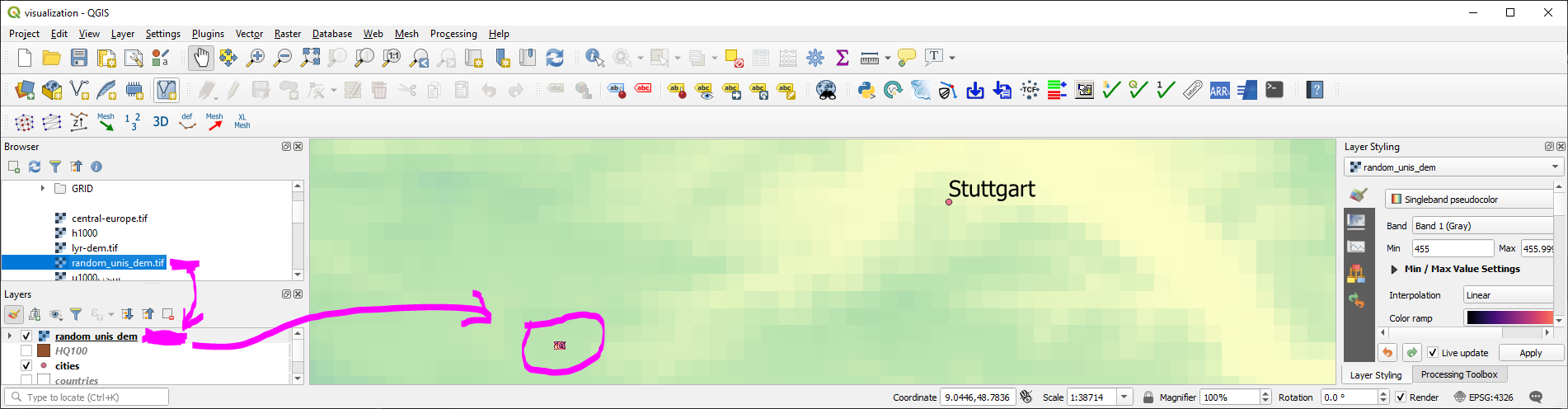
Figure 1:Das neue Raster mit einer zufälligen unis dem-Punkthöhe.
Rasterkalkulus (Raster / Band zum Array)
Das mit der Funktion create_raster() beschriebene Verfahren kann umgekehrt verwendet werden, um numpy array aus Rasterbändern zu erstellen. Das in ein Numpy-Array konvertierte Raster ermöglicht es, algebraische oder andere logische Operationen auf vorhandene Rasterdaten anzuwenden.
Need an example? In the RiverArchitect SampleData, the units of the water depth raster h001000.tif are in U.S. customary feet and the units of the flow velocity raster u001000.tif are in feet per second. However, to calculate the Froude-Zahl (involves the gravity constant) for every pixel based on the two rasters (water depth and flow velocity), it is convenient to convert both rasters into m and m/s, respectively. For this purpose, the following code block features another re-usable, custom function that loads a raster as an array and overwrites NoDataValues with np.nan (raster and band can be instantiated with the above open_raster function):
def raster2array(file_name, band_number=1):
    """
    :param file_name: STR of target file name, including directory; must end on ".tif"
    :param band_number: INT of the raster band number to open (default: 1)
    :output: (1) ndarray() of the indicated raster band, where no-data values are replaced with np.nan
             (2) the GeoTransformation used in the original raster
    """
    # open the raster and band (see above)
    raster, band = open_raster(file_name, band_number=band_number)
    # read array data from band
    band_array = band.ReadAsArray()
    # overwrite NoDataValues with np.nan
    band_array = np.where(band_array == band.GetNoDataValue(), np.nan, band_array)
    # return the array and GeoTransformation used in the original raster
    return raster, band_array, raster.GetGeoTransform()
Die Funktion raster2array() ist auch in flusstools enthalten: geotools.raster2array()
Finally, to create a Froude number GeoTIFF raster, the following code block makes use of the raster2array function for converting the water depth and flow velocity GeoTIFF rasters into a numpy array, performing simple algebraic calculations to convert the rasters to m and m/s, respectively, and save the resulting GeoTIFF file. In detail, the workflow involves to:
Definieren Sie die Eingabe-Raster-Dateinamen mit Verzeichnissen (
h_fileundu_file),Load original rasters as
ndarraywith theraster2array()function and get the originalGeoTransformdescription,Convert all values from U.S. customary feet to S.I. metric units (recall the feet_to_meter() function from the Python basics), and
Speichern Sie eine neue Kopie des Rasters.
h_file = r"" + os.getcwd() + "/geodata/rasters/h001000.tif"
u_file = r"" + os.getcwd() + "/geodata/rasters/u001000.tif"

# load both rasters as arrays
h_ras, h, h_geo_info = raster2array(h_file)
u_ras, u, u_geo_info = raster2array(u_file)

#convert to metric system
h *= 0.3048
u *= 0.3048

# calculate the Froude number as array and avoid zero-division warning messages
with np.errstate(divide="ignore", invalid="ignore"):
    Froude = u / np.sqrt(h * 9.81)

# create Froude raster from array
create_raster(file_name= r"" + os.path.abspath("") + "/geodata/rasters/Fr1000cfs.tif",
              raster_array=Froude, epsg=6418, geo_info=h_geo_info)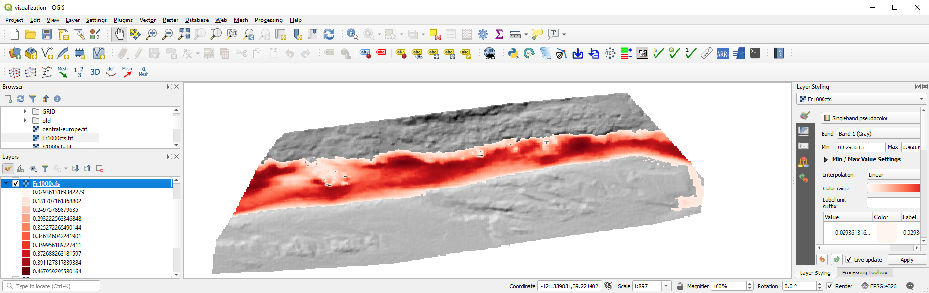
Figure 2:Das Froude-Zahlenraster wird mit Strömungsgeschwindigkeits- und Wassertiefenrastern berechnet.
Reproject a raster
Die Transformation (und Reprojektion) eines Rasters in ein anderes Koordinatensystem beinhaltet das Drehen, Verschieben und Scheren von Pixeln. Wenn eine dieser Operationen übersprungen wird, kann das neu projizierte Raster gequetscht, verdreht oder irgendwo in der Welt platziert werden, aber nicht dort, wo es platziert werden sollte. Der Ansatz zur Reprojektion eines Rasters in ein anderes Koordinatenreferenzsystem beinhaltet daher folgende Schritte:
Retrieve the source and target spatial reference systems (e.g., derive from a
gdal.Datasetor anEPSGauthority code).Lesen Sie die Geo-Transformation des Quelldatensatzes (
gdal.Dataset.GetGeoTransform()).Ableiten der Anzahl der Pixel und des Abstands zwischen den Pixeln im neuen (reprojizierten) Datensatz.
Instantiieren Sie den neuen (reprojizierten) Datensatz.
Projizieren Sie ein Bild des Quelldatensatzes auf den neuen (reprojizierten) Datensatz (
gdal.ReprojectImage()).
Das räumliche Bezugssystem kann aus einem Datensatz mit den Erklärungen im Abschnitt shapefile abgeleitet werden, indem eine get_srs()-Funktion geschrieben wird. Der folgende Codeblock zeigt die get_srs()-Funktion (verwendet die osr-Bibliothek von osgeo / gdal ), die ebenfalls in flusstools @ geotools.get_srs()] integriert ist.
def get_srs(dataset):
    """
    Get the spatial reference of any gdal.Dataset
    :param dataset: osgeo.gdal.Dataset (raster)
    :output: osr.SpatialReference
    """
    sr = osr.SpatialReference()
    sr.ImportFromWkt(dataset.GetProjection())
    # auto-detect epsg
    auto_detect = sr.AutoIdentifyEPSG()
    if auto_detect != 0:
        sr = sr.FindMatches()[0][0]  # Find matches returns list of tuple of SpatialReferences
        sr.AutoIdentifyEPSG()
    # assign input SpatialReference
    sr.ImportFromEPSG(int(sr.GetAuthorityCode(None)))
    return sr
With the open_raster() and get_srs() functions, we have all necessary ingredients to accomplish the raster reprojection workflow in another function called reproject_raster(). An additional feature of the function is that it ensures the correct use of osr.CoordinateTransformation, which behaves differently under gdal 3.0 compared with older gdal versions (read more on OSGeo’s GitHub page).
def reproject_raster(source_dataset, source_srs, target_srs):
    """
    Reproject a raster dataset to an in-memory warped VRT.
    :param source_dataset: osgeo.gdal.Dataset (instantiate with gdal.Open(RASTER-FILE))
    :param source_srs: osgeo.osr.SpatialReference (instantiate with get_srs(source_dataset))
    :param target_srs: osgeo.osr.SpatialReference for the target CRS
    """
    # use traditional GIS axis order for GDAL 3 and later
    source_srs.SetAxisMappingStrategy(osr.OAMS_TRADITIONAL_GIS_ORDER)
    target_srs.SetAxisMappingStrategy(osr.OAMS_TRADITIONAL_GIS_ORDER)


    return gdal.AutoCreateWarpedVRT(
        source_dataset,
        source_srs.ExportToWkt(),
        target_srs.ExportToWkt(),
        gdal.GRA_Bilinear,
    )
Using the reproject_raster() function in a Python script requires a source dataset and another (orientation) dataset with the new coordinate system into which the source dataset will be projected. The following example shows how to re-project the above-created Froude-number raster into the EPSG=3857 coordinate system for viewing it in QGIS on a Google Satellite basemap (recall basemaps in QGIS tutorial). As orientation data set, use web_frame.tif, which was created on the Google Satellite basemap.
Mit der Funktion get_srs(), die das Rasterprojektions- und räumliche Referenzsystem automatisch erkennt, können wir die Funktion create_raster() verwenden, um das oben erstellte Fr1000cfs.tif-Raster neu zu projizieren (z. B. auf epsg=4326).
# load original and orientation rasters
source_file_name = r"" + os.path.abspath("") + "/geodata/rasters/Fr1000cfs.tif"
orientation_file_name = r"" + os.path.abspath("") + "/geodata/rasters/web_frame.tif"

src_dataset, src_band = open_raster(source_file_name)
ort_dataset, ort_band = open_raster(orientation_file_name)

src_srs = get_srs(src_dataset)
new_srs = get_srs(ort_dataset)

print("Source EPSG: " + str(src_srs.GetAuthorityCode(None)))
print("Target EPSG: " + str(new_srs.GetAuthorityCode(None)))

# flush orientation dataset
ort_dataset, ort_band = None, None

# create re-projected raster and save as GeoTIFF
reproj_dataset = reproject_raster(src_dataset, src_srs, new_srs)
reproj_file_name = r"" + os.path.abspath("") + "/geodata/rasters/Fr1000cfs_reproj.tif"
array_data = reproj_dataset.ReadAsArray()
new_epsg = int(new_srs.GetAuthorityCode(None))
geo_transformation = reproj_dataset.GetGeoTransform()
create_raster(reproj_file_name, raster_array=array_data, epsg=new_epsg, geo_info=geo_transformation)
reproj_dataset = None
Source EPSG: 6418
Target EPSG: 3857
Aufgetragen in QGIS, sieht das neu projizierte Froude-Zahlen-Raster so aus:
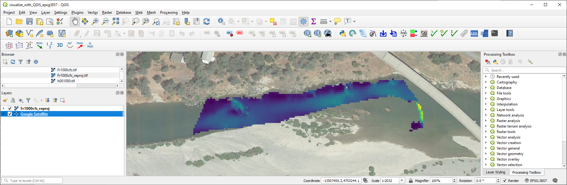
Figure 3:Das projizierte Raster von Froude Zahlen.
Die Funktion reproject_raster ist auch in flusstools (geotools.reproject_raster()) verfügbar (geringfügig modifiziert), wo das Speichern des neu projizierten Rasters in die Funktion eingebettet ist (automatisch fügt die Silbe "_epsg[NO]" an den ursprünglichen Dateinamen an).
Zonal Statistiken für morphologische Einheiten
In hydraulischen und geospatialen Analysen stellt sich oft die Frage nach statistischen Werten bestimmter Bereiche eines oder mehrerer Raster. Zum Beispiel könnten uns Mittelwerte und Standardabweichungen in bestimmten Zonen eines Gewässers interessieren. Zu diesem Zweck ermöglichen Zonale Statistiken die Abgrenzung eines Bereichs eines Rasters unter Verwendung eines Polygon-Shapefiles.
Der River Architect-Datensatz enthält eine Slackwater-Zone und zonale Statistiken helfen, die mittlere Wassertiefe und Strömungsgeschwindigkeit von Slackwaters zu identifizieren, die eine sogenannte morphologische Einheit (recall the create-shapefile section) sind.
Um eine visuell sichtbare Slackwater-Einheit zu analysieren, können wir ein Polygon in ein neues Shapefile zeichnen, das morphologische Einheiten beschreibt. Die folgenden Figuren führen durch die Erstellung eines Polygon-Shapefiles und die Abgrenzung des Riffles mit QGIS. Beginnen Sie mit dem Öffnen von QGIS und erstellen Sie ein neues Projekt. Importieren Sie die Wassertiefe und Strömungsgeschwindigkeit Raster der langsamen und flachen Wasserzone. Folgen Sie dann dem Workflow in den Abbildungen unten.
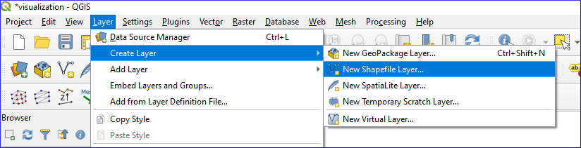
Figure 4:QGIS: Layer erstellen > New Shapefile Layer...
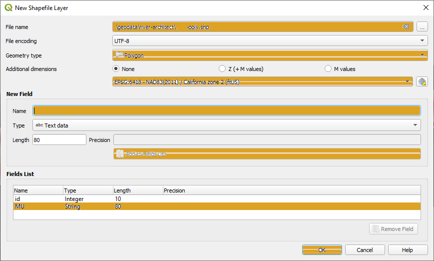
Figure 5:Definieren Sie neue Shapefile Layer

Figure 6:Shapefile Editing aktivieren
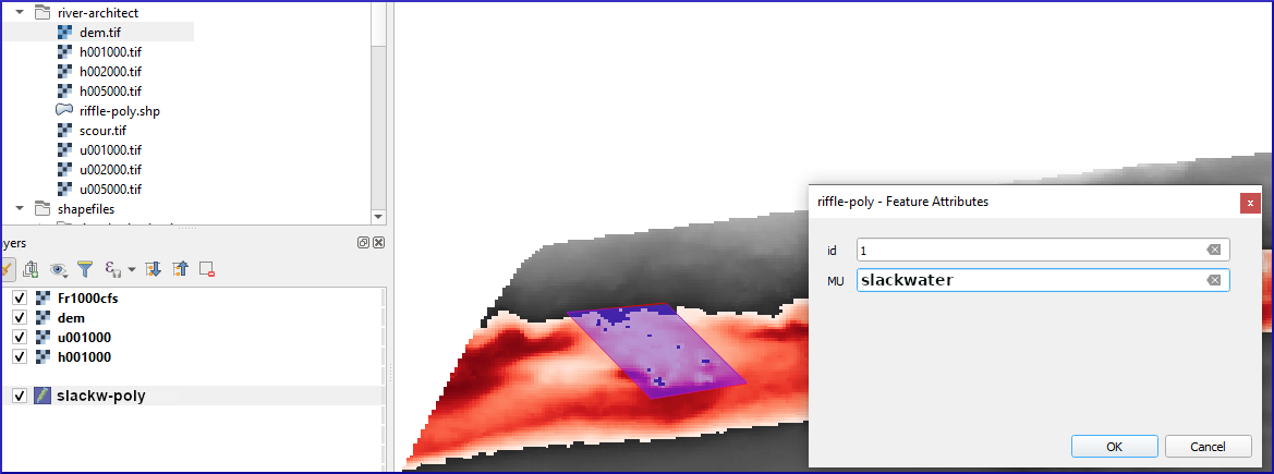
Figure 7:Zeichne Polygone in einer Shapefile in QGIS.
Schließen Sie die Zeichnung ab, indem Sie auf die Schaltfläche Bearbeiten speichern klicken (zwischen Toggle Editing und Polygon hinzufügen). Nur für den Fall, die Slackwater Delineation Polygon Shapefile ist auch verfügbar unter das Jupyter-python repository dieses eBook].
Zonal statistics can be calculated using the gdal and ogr libraries, but this is a little cumbersome. The rasterio (conda install -c conda-forge rasterio) library provides a much more convenient method to calculate zonal statistics with its rasterstats.zonal_stats(SHP-FILE, RASTER, STATISTICS-TYPES) method. With zonal_stats, we can easily obtain statistics of the water depth and flow velocity rasters in the limits of the new slackwater polygon.
import rasterstats as rs
# make file names
h_file = r"" + os.getcwd() + "/geodata/rasters/h001000.tif"
u_file = r"" + os.getcwd() + "/geodata/rasters/u001000.tif"
zone = r"" + os.getcwd() + "/geodata/shapefiles/slackw-poly.shp"

# get water depth stats in zone
h_stats = rs.zonal_stats(zone, h_file, stats=["min", "max", "median", "majority", "sum"])
# get flow velocity stats in zone - note the different stats assignment
u_stats = rs.zonal_stats(zone, u_file, stats="min max median majority sum")

print(h_stats)
print(u_stats)
[{'min': 0.0, 'max': 5.423915386199951, 'sum': 1709.34521484375, 'median': 1.6403688192367554, 'majority': 0.0}]
[{'min': 0.0, 'max': 5.139162540435791, 'sum': 1609.26318359375, 'median': 1.879171371459961, 'majority': 0.0}]
Daran erinnern, dass beide Raster in der US-üblichen Einheit System (dh Füße und Füße pro Sekunde) sind. Weitere Statistiken können mit zonal_stats berechnet werden:
min, max, mean, count, sum, std, median, majority, minority, unique, range, nodata, percentile_<q> (wobei <q> eine beliebige Float-Nummer zwischen 0 und 100 sein kann).
Darüber hinaus können benutzerdefinierte Statistiken hinzugefügt werden, wobei das Modul numpy.ma] mit seinen Array-Handling-Kapazitäten besonders nützlich ist, z. B. zum Transponieren oder Spezifizieren von Statistiken entlang einer Achse. Zum Beispiel können wir eine bestimmte Funktion definieren, um die Standardabweichung wie folgt zu berechnen:
def raster_std(raster_array):
    return np.ma.std(raster_array)
Um die Funktion raster_std in zonal_stats zu verwenden, schreiben Sie etwas Ähnliches:
u_stats = rs.zonal_stats(
    zone, u_file,
    stats="min max",
    add_stats={"stdev": raster_std}
)
print(u_stats)
[{'min': 0.0, 'max': 5.139162540435791, 'stdev': np.float64(1.1065991101701524)}]
Clip a raster
The above-introduced rasterstats.zonal_stats method works with “Mini-Rasters”, which represent clips of the input raster to the user-defined polygon shapefile. Moreover, a mini-raster itself can be obtained by defining the optional keyword argument raster_out=True. In the case that we want to get the original raster clipped without and statistical operation, we can use a little trick by defining an additional statistics function that returns the original array:
def original(raster_array):
    return raster_array
Mit raster_out=True und der Funktion original() können wir das beschnittene Raster in den folgenden Array-Typen abrufen:
mini_raster_array- ein beschnittenes und maskiertes Numpy-Array,mini_raster_affine- eine Transformation alsAffine-Objekt (d.h. mit affine 6-Parameter-Transformation]), undmini_raster_nodata-NoDataWerte.
Der folgende Codeblock veranschaulicht die Verwendung zum Abrufen eines Numpy-Arrays:
import rasterstats as rs

h_file = r"" + os.getcwd() + "/geodata/rasters/h001000.tif"
h_stats = rs.zonal_stats(zone, h_file, stats="count",
                         add_stats={"original": original},
                         raster_out=True)
print(h_stats[0].keys())
print(h_stats[0]["mini_raster_array"])
dict_keys(['count', 'original', 'mini_raster_array', 'mini_raster_affine', 'mini_raster_nodata'])
[[-- -- -- ... -- -- --]
[-- -- -- ... -- -- --]
[-- -- -- ... -- -- --]
...
[-- -- -- ... -- -- --]
[-- -- -- ... -- -- --]
[-- -- -- ... -- -- --]]
Slope / Seitenkarten und integrierte Kommandozeilenskripte
Hillslope maps are an important parameter in hydraulics, hydrology, and ecology. For instance, the slope determines the flow direction of water and it is also a criterion for delineating the habitat of many species. To calculate hill slope gradients and directions, gdal has a command-line tool called gdaldem , which requires a DEM (Digital Elevation Model) raster. The general use of gdaldem in the command line is (arguments in brackets are optional):
gdaldem slope input_dem output_slope_map [-p use percent slope (default=degrees)] [-s scale* (default=1)] [-alg ZevenbergenThorne] [-compute_edges] [-b Band (default=1)] [-of format] [-co "NAME=VALUE"]* [-q]To call the command-line tool, we can either use a terminal/command prompt or Python’s standard library subprocess. The following code block illustrates the usage of the gdaldem command line tool through subprocess.call() to create a slope raster (in percent) from the River Architect sample data’s dem.tif. Note that subprocess.call() returns 0 if the command execution was successful and any other return value indicates an error.
import subprocess, os

cmd_create_slope = "gdaldem slope {0}/geodata/rasters/dem.tif {0}/geodata/rasters/slope-percent.tif -p".format(os.path.abspath(""))
subprocess.call(cmd_create_slope, shell=True)
0...10...20...30...40...50...60...70...80...90...100 - done.
0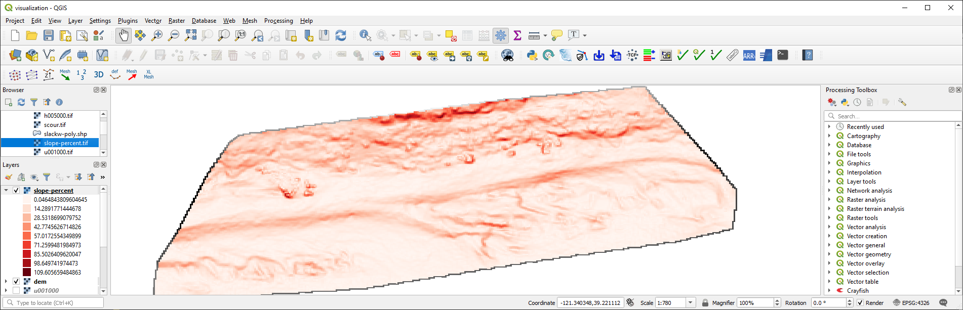
Figure 8:Das neue Pistenraster.
Zusätzlich zur absoluten Steigung (d.h. Neigung in Grad) oder anstelle der Steigung kann es wichtig sein, die Steigungsrichtung zu kennen (z.B. Neigung nach Süden, Westen, Osten oder Norden). Ein Raster, das die Hangrichtung anzeigt, wird als aspect raster bezeichnet, wobei Süden 0° (und 360°), Westen 90°, Norden 180° und Osten 270° entspricht. Ein Aspektraster kann auch mit gdaldem erstellt werden:
gdaldem aspect input_dem output_aspect_map [-trigonometric] [-zero_for_flat] [-alg ZevenbergenThorne] [-compute_edges] [-b Band (default=1)] [-of format] [-co "NAME=VALUE"]* [-q]Um ein Aspektraster der River Architect Beispieldaten Digitales Oberflächenmodell (DOM) run zu erstellen:
cmd_create_aspect = "gdaldem aspect {0}/geodata/rasters/dem.tif {0}/geodata/rasters/slope-aspect.tif".format(os.path.abspath(""))
subprocess.call(cmd_create_aspect, shell=True)
0...10...20...30...40...50...60...70...80...90...100 - done.
0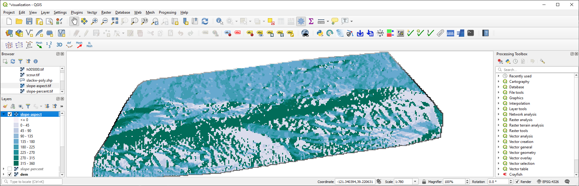
Figure 9:Der neue Aspekt Raster.
Least Cost path zwischen Pixeln (und einer anderen Art von Reprojektion)
Ökohydraulik Hintergrund
Kostengünstigste Pfade sind wichtig, um effiziente Routen für die Navigation zu planen (z. B. in einem Auto), und sie können auch in der Ökohydraulik hilfreich sein. Nehmen wir für einen Moment die Position eines Fisches, der nach einer Flut mit abnehmender Entladung so schnell wie möglich aus der Aue zurück in den Hauptkanal schwimmen möchte, wo es genug Wasser gibt. In der folgenden Abbildung zeigt Punkt 1 den Startpunkt auf der Aue und Punkt 2 das Ziel im Hauptkanal. Der rötliche Hintergrund stellt das oben erzeugte Hangraster (slope-percent.tif) dar und die Wassertiefe ist bei durchschnittlichem Jahresaustrag blau eingefärbt.
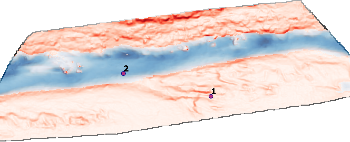
Figure 10:Das Steigungsraster mit den Punkten 1 und 2 hervorgehoben.
Natürlich entspricht der Weg der geringsten Kosten dem Weg des steilsten, monoton nach unten gerichteten Hangs, und wir werden davon ausgehen, dass ein Fisch ihn finden kann.
Funktionen und Bibliotheken beteiligt
The skimage (scikit-image) library (cf. Other packages in the Open source libraries section) provides with skimage.graph.route_through_array a smart method to calculate the least cost path by summing up pixel-wise connections from point 1 to point 2.
Hier ist, wie es funktioniert: Angenommen, ein numpy-array (z. B. mit zufälligen Steigungswerten), das so aussieht:
slope_image = np.random.randint(100, size=(3, 5))
slope_image
array([[43, 68, 67, 88, 60],
[22, 95, 90, 97, 0],
[38, 18, 83, 65, 83]])Um den schnellsten Weg vom Array-Index [0][0] (oben links point_1 = (0, 0)) zum Array-Index [2][4] (unten rechts point_2 = (2, 4)) zu finden, können wir route_through_array() verwenden, um eine *Liste * (least_cost_path_indices) mit den Array-Koordinaten des zu gehenden Pfades und den damit verbundenen Kosten (weight) zu erhalten (Summe aller Pixel des kostengünstigsten Pfades):
from skimage.graph import route_through_array

point_1 = (0, 0)
point_2 = (2, 4)
least_cost_path_indices, weight = route_through_array(slope_image, point_1, point_2)
least_cost_path_indices, weight
([(0, 0), (1, 0), (2, 1), (2, 2), (2, 3), (2, 4)],
np.float64(259.2842712474619))Um die Liste der kostengünstigsten Pfade in ein Array zu integrieren, das wir rasterisieren (geotools.create_raster()), können wir least_cost_path_indices in ein Numpy-Null-Array des ursprünglichen Steigungsrasters (Bild) als transponierte Liste einfügen.
least_cost_path_indices = np.array(least_cost_path_indices).T
least_cost_path_array = np.zeros_like(slope_image)
least_cost_path_array[least_cost_path_indices[0], least_cost_path_indices[1]] = 1
least_cost_path_array
array([[1, 0, 0, 0, 0],
[1, 0, 0, 0, 0],
[0, 1, 1, 1, 1]])In der Praxis wird das Steigungsraster georeferenziert, und deshalb müssen wir Pixelkoordinaten relativ zum Koordinatensystem-Ursprung verwenden. Dazu benötigen wir zwei weitere Funktionen:
One function to calculate the pixel-index related offset that we will name
coords2offset: Thecoords2offset()function will return the x-y shift in the form of “number of pixels” (two integers, one for x and one for y shift).Die Funktion above-defined get_srs() (d.h.
geotools.get_srs()).
Die Funktion coords2offset() sieht so aus:
def coords2offset(geo_transform, x_coord, y_coord):
    """
    Returns x-y pixel offset
    :param geo_transform: osgeo.gdal.Dataset.GetGeoTransform() object
    :param x_coord: FLOAT of x-coordinate
    :param y_coord: FLOAT of y-coordinate
    :return: offset_x, offset_y (both integer of pixel numbers)
    """
    origin_x = geo_transform[0]
    origin_y = geo_transform[3]
    pixel_width = geo_transform[1]
    pixel_height = geo_transform[5]
    offset_x = int((x_coord - origin_x) / pixel_width)
    offset_y = int((y_coord - origin_y) / pixel_height)
return offset_x, offset_yThe coords2offset() function converts a raster array (e.g., produced with the above-defined geotools.raster2array() function) into an array that can be used with route_through_array() with the following workflow:
Verwenden Sie die Raster-
geo_transform(gdal.Dataset.GetGeoTransform = (origin_x, pixel_width, 0, origin_y, 0, pixel_height)) und die Start- und Endpunktkoordinaten (dhstart_coordvon Punkt 1 undstop_coordvon Punkt 2) incoords2offset(), um ihre Pixelindizes (start_index_x,start_index_y,stop_index_xundstop_index_y) im Raster-Array zu erhalten.Replace
np.nanvalues in the raster array with values that are higher than the maximum value of the array. Do not use zeros, because we want to exclude thenp.nanpixels from the least cost path later by overwritingnp.nanwith very high pixel costs.Verwenden Sie
route_through_array()wie oben mit den optionalen Argumentengeometric=Trueerklärt (verwenden Sie die MCP Geometric class statt MCP base, um Kosten zu berechnen) undfully_connected=True(ermöglicht die Verwendung diagonaler Pixel als direkte Nachbarn).Integrieren Sie die Liste der kostengünstigsten Pfade (
index_path) in ein Numpy-Null-Array (Kind vonraster_array, wie oben erläutert) und geben Siepath_arrayzurück.
def create_path_array(raster_array, geo_transform, start_coord, stop_coord):
    # transform coordinates to array index
    start_index_x, start_index_y = coords2offset(geo_transform, start_coord[0], start_coord[1])
    stop_index_x, stop_index_y = coords2offset(geo_transform, stop_coord[0], stop_coord[1])

    # replace np.nan with max raised by an order of magnitude to exclude pixels from least cost
    raster_array[np.isnan(raster_array)] = np.nanmax(raster_array) * 10

    # create path and costs
    index_path, cost = route_through_array(raster_array, (start_index_y, start_index_x),
                                               (stop_index_y, stop_index_x),
                                               geometric=True, fully_connected=True)


    index_path = np.array(index_path).T
    path_array = np.zeros_like(raster_array)
    path_array[index_path[0], index_path[1]] = 1
return path_arrayAntragstellung
Erinnern Sie sich, wir haben die folgenden Funktionen definiert (alle sind in flusstools bis from flusstools import geotools] verfügbar), die wir für die Berechnung des kostengünstigsten Pfades verwenden können, um von Punkt 1 nach Punkt 2 im Raster *slope-percent.tif * zu gelangen:
geotools.raster2array()geotools.create_path_array()geotools.get_srs()geotools.create_raster()
Der folgende Codeblock verwendet diese Funktionen wie folgt:
Definieren Sie Input (slope-percent.tif) und Output (least cost.tif) Rasternamen (mit Verzeichnissen).
Definieren Sie die Koordinaten der Punkte 1 und 2 als Tupels (x, y) in der EPSG:6418 Projektion.
Laden Sie das Eingaberaster (
src_raster), sein Band als Array (raster_array) und die Geotransformation (geo_transform) mit der Funktionraster2array().Get the least cost path indicated with ones in an array of zeros ( i.e., an on-off
path_array) with thecreate_path_array()function.Holen Sie sich das
osgeo.osr.SpatialReferencedes Eingaberasters (src_raster = osgeo.gdal.Dataset("slope-percent.tif")).Create the least cost path GeoTIFF raster with the
create_raster()function as agdal.GDT_Byteband.
from skimage.graph import route_through_array

# define raster input and out names
in_raster_name = r"" + os.path.abspath("") + "/geodata/rasters/slope-percent.tif"
out_raster_name = r"" + os.path.abspath("") + "/geodata/rasters/least_cost.tif"
# define coordinates of points 1 and 2 (in EPSG:6418)
point_1_coord = (6749261.94092826917767525, 2206970.35179582564160228)
point_2_coord = (6749016.82820663042366505, 2207050.61491037486121058)

# get source raster (osgeo.gdal.Dataset), the raster as nd.array, and the geotransformation tuple
src_raster, raster_array, geo_transform = raster2array(in_raster_name)
# get the zeros-like array with least cost pixels = 1
path_array = create_path_array(raster_array, geo_transform, point_1_coord, point_2_coord)
# get the spatial reference system of the input raster (slope-percent.tif)
src_srs = get_srs(src_raster)
# project the least cost path_array into a Byte (only zeros and ones) raster
create_raster(out_raster_name, path_array, epsg=int(src_srs.GetAuthorityCode(None)),
              rdtype=gdal.GDT_Byte, geo_info=geo_transform)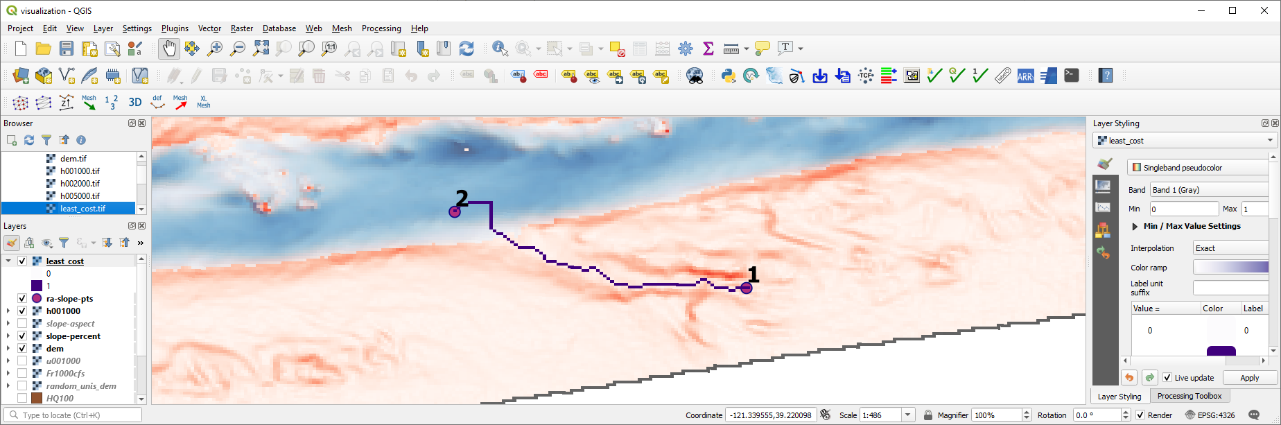
Figure 12:Der in QGIS dargestellte Weg mit den geringsten Kosten.
Legitimately, you may wonder whether it was better to represent the least cost path as a line. Of course, that is correct. However, this operation is a conversion of a raster into a line shapefile, which is explained in the next section on geodata conversion. Curious readers can also directly use the raster2line() function of flusstools (or have a look at it in the flusstools
- Wyrick, J. R., & Pasternack, G. B. (2014). Geospatial organization of fluvial landforms in a gravel-cobble river: Beyond the riffle-pool couplet. Geomorphology, 213(Supplement C), 48–65. 10.1016/j.geomorph.2013.12.040
- Schwindt, S., Larrieu, K., Pasternack, G. B., & Rabone, G. (2020). River Architect. SoftwareX, 11, 100438. 10.1016/j.softx.2020.100438