Geodatenquellen¶
Geodaten können für verschiedene Zwecke aus verschiedenen Quellen abgerufen werden. Hier sind einige davon:
Geografische Kartendaten im Atlas-Stil werden von naturalearthdata
.com] bereitgestellt (z. B. die ~230 MB Natural Earth Quick Start Kit gebündelt mit vorgefertigten QGIS-Projekten]. Digitales Oberflächenmodells, ozeanographische und weitere wasserbezogene Karten sind unter den USA verfügbar NOAA Geo-platform und seine TDS Catalog]
OpenStreetMap data extractions are available at https://
download .geofabrik .de/ Satellitenbilder sind verfügbar unter
[USGS] Earth Explorer](https://
earthexplorer .usgs .gov/) ESA Copernicus Data Space Ecosystem (Sentinel-1/2/3/5P; diese ersetzte den ehemaligen Copernicus Open Access Hub / SciHub, der am 2. November 2023 stillgelegt wurde]
planet.com (kommerziell)]
LiDAR Daten finden Sie unter opentopography.org].
Klimatologische Daten werden von NASA Earth Observations (NEO) bereitgestellt.
Meteorologische (z. B. Temperatur oder Niederschlag) und Echtzeit-Satellitendaten sind unter wunderground.com und dessen wundermap] verfügbar.
Klima- und Wetterdaten und -vorhersagen sind unter cds
.climate .copernicus .eu verfügbar, einschließlich z. B. ERA5 monatlich gemittelte Temperaturdaten] Daten zur Landnutzung (einschließlich Baumkronenabdeckung), sozioökonomischen Merkmalen und globalen Veränderungen sind im FAO-Kartenkatalog (GeoNetwork) oder im archivierten ISCGM Global Map-Portal (gehen Sie zu ihrem GitHub-Archiv].]
Topographical data (1 to 5-m resolution) from the state of Bavaria, Germany, can be found at https://
www .ldbv .bayern .de. Topographical data from EU countries can be found at https://
www .mapsforeurope .org.
Visualisierung¶
GIS software is needed to display geospatial data and many tools exist. This website primarily provides examples using QGIS. Since the use of GIS software, especially QGIS, is necessary for several sections in this eBook, explanations on how to install QGIS are already included in the Geodatensoftware.
Geodatenbank¶
Eine Geodatenbank (auch bekannt als spatial database) kann speichern, abfragen (z. B. unter Verwendung von Structured Query Language SQL]) oder Daten mit geografischen Referenzen ändern (geospatial data). Geodaten bestehen in erster Linie aus Vektordaten (siehe Shapefiles), es können aber auch Rasterdaten implementiert werden. Eine Geodatenbank verknüpft diese Daten mit Attributtabellen und geografischen Koordinaten. Eine Besonderheit von Geodatenbanken ist, dass sie über einen (Web- oder lokalen) GIS-Server (Geographic Information System) visualisiert und manipuliert werden können. Zum Beispiel ermöglicht Software wie QGIS (oder ArcGIS Pro) das Erstellen von Karten und Abfragen auf einer Art lokalem Server mit lokal gespeicherten Geodaten. Das typische Geodatenbankformat ist .gdb, das als Verzeichnis in QGIS oder ArcGIS funktioniert, und die maximale Größe einer .gdb-Datei beträgt 1 Terabyte.
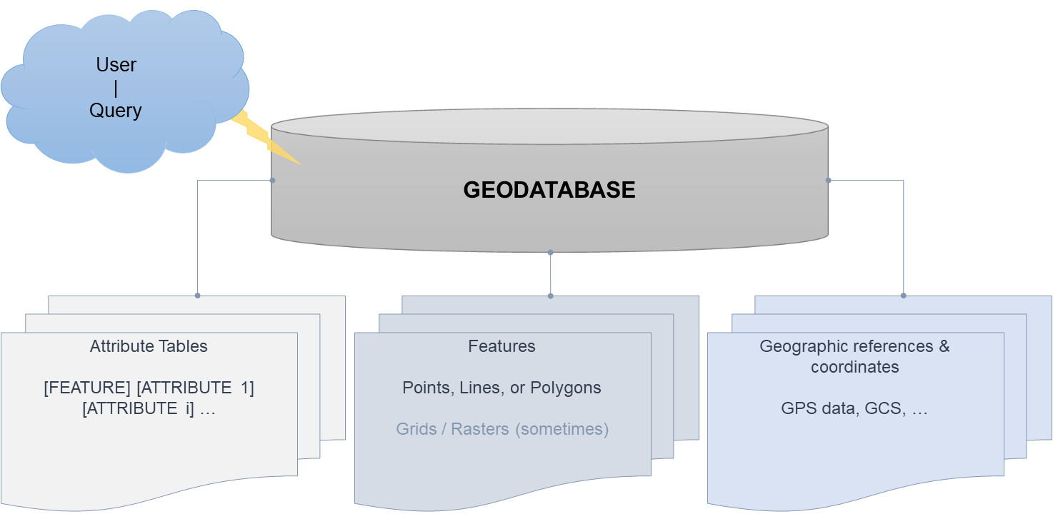
Das funktionale Skelett einer Geodatenbank.
Vektordaten¶
Vektordaten sind optisch glatt und effizient für Überlagerungsoperationen, insbesondere in Bezug auf formgesteuerte Geoinformationen wie Straßen oder Oberflächenabgrenzungen. Vektordaten werden als wenig speicherintensiv, einfach zu skalieren und mit relationalen Umgebungen kompatibel charakterisiert. Gängige Formate sind .shp, JSON oder TIN.
Das Shapefile-Format wurde von Esri in den frühen 1990er Jahren erfunden (das Original shapefile technical description (PDF) bleibt die maßgebliche Referenz) und die in einer Shapefile enthaltenen Informationen können sein:
Polygone (Oberflächenflecken),
Punkte mit x-y-z-Koordinaten und einem m-Feld mit Punktdaten und
(Poly) Linien, die aus Linien bestehen, die durch Startpunkte und Endpunkte definiert sind.
Shapefil¶
Eine Shapefile besteht aus mehreren Dateien auf der Festplatte mit den folgenden wesentlichen Teilen:
eine
.shp-Datei, in der Geometrien gespeichert sind,eine
.shx-Datei, in der Indizes der Geometrien gespeichert sind,a
.prjfile that stores the projection, andeine
.dbf-Datei mit Attributinformationen (bildet die Attributtabelle).
These files need to be in the same folder - otherwise, the shapefile is incomplete and does not work (correctly). A couple of other files may occur when we manipulate a shapefile (e.g., .atx, .sb*, .shp.xml, .cpg, .mxs, .ai*, or .fb*), but we can ignore those files.
Shapefile-Vektordaten haben typischerweise eine Attributtabelle (wie jede andere Geodatenbank), in der jedem Polygon, jeder Linie oder jedem Punktobjekt ein Attributwert zugewiesen werden kann. Attribute werden durch Spalten zusammen mit ihren Namen (Spaltenüberschriften) definiert und können numerische Formate (z.B. float, double, int oder long), Text (string) oder Datum/Uhrzeit (z.B. yyyymmdd oder HH:MM:SS) haben.
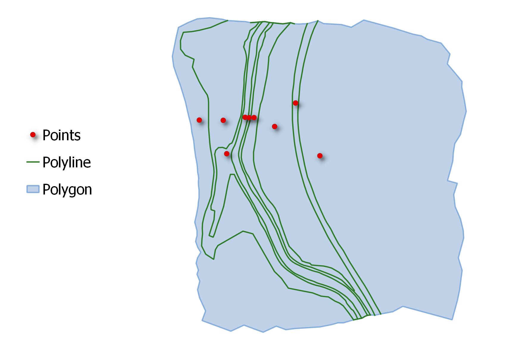
Darstellung von Punkt (rot), (Poly) Linie (grün) und Polygon (blau) Shapefile Features.
Shapefile versus Geodatabase¶
Eine Shapefile kann als Konkurrenzformat zu einer Geodatenbank verstanden werden. Welches Dateiformat ist besser? Streng genommen können sowohl eine Geodatenbank als auch eine Shapefile ähnliche Operationen ausführen, aber eine Shapefile benötigt mehr Speicherplatz zum Speichern ähnlicher Inhalte, kann keine kombinierten Datums- und Zeitfelder speichern und unterstützt keine Rasterdaten oder Null (not-a-number) Werte. Shapefiles sind auch auf 2 GB pro Komponentendatei, Attributnamen von 10 Zeichen oder weniger und Textfelder von 255 Zeichen oder weniger begrenzt. Daher haben Geodatenbanken (und das portablere GeoPackage-Format) einen technischen Vorteil gegenüber Shapefiles, aber die Verwendung von Shapefiles ist immer noch beliebt und viele ältere Geodaten-Workflows konzentrieren sich auf Shapefil-Manipulationen.
Trianguliertes unregelmäßiges Netzwerk (TIN)¶
A triangulated irregular network (TIN) represents a surface composed of multiple triangles. In hydraulic engineering and water resources research, one of the most important uses of a TIN is the generation of computational meshes for numerical models (read more in the GRUNDLAGE tutorial, for example). In such models, a TIN consists of lines and nodes forming georeferenced, three-dimensionally sloped triangles of the surface, which represent a digital elevation model (DEM). TIN nodes have georeferenced coordinates and potentially more attribute information such as node IDs and elevation. The advantage of a TIN DEM over a raster (see below) DEM is that it requires less storage space. However, manipulating a TIN is not as straightforward as manipulating a raster. The below figure shows an example TIN created with matplotlib.tri.TriAnalyzer, and based on a showcase from the matplotlib docs. The file ending of a TIN is .tin.
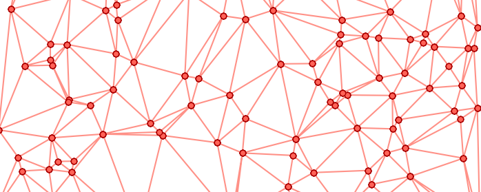
Illustration einer TIN.
GeoJSON¶
GeoJSON ist ein offenes Format zur Darstellung geografischer Daten mit einfachen Feature-Zugriffsstandards, wobei JSON JavaScript Object Notation bezeichnet (lesen Sie mehr über JSONDateimanipulation in den Python-Grundlagen). GeoJSON ist standardisiert als RFC 7946]. Das Ende des GeoJSON-Dateinamens ist .geojson und eine Datei hat normalerweise die folgende Struktur:
{
  "type": "FeatureCollection",
  "features": [
    {
      "type": "Feature",
      "geometry": {
        "type": "Point",
        "coordinates": [9.104028940200806, 48.74417005744522]
      },
      "properties": {
        "name": "IWS"
      }
    }
  ]
}
While GeoJSON metadata can provide height information (z values) as a properties value, there is a more suitable offspring to encode geospatial topology in the form of the TopoJSON format. To manipulate GeoJSON files with Python, go to the Geojson section. To build a customized GeoJSON file, visit geojson.io.
GeoPackage (GPKG)¶
GeoPackage (.gpkg) ist ein offenes, plattformunabhängiges, standardbasiertes Geodatenformat, das vom Open Geospatial Consortium (OGC) (OGC-Standard 12-128r19) veröffentlicht wird.] Technisch gesehen ist ein GeoPackage eine einzige SQLite3 Datenbankdatei, die der GeoPackage-Spezifikation folgt, was bedeutet, dass es mit jedem SQLite-basierten Tool zusätzlich zu GIS-Software wie QGIS geöffnet, abgefragt und geändert werden kann.
In contrast to a shapefile (which is really a small bundle of sidecar files), a GeoPackage is one single file that can simultaneously contain:
Mehrere **Vektorenschichten (Punkte, Linien, Polygone, Mischgeometrie) in einem Behälter,
Raster Fliesenpyramiden (z.B. GeoTIFF-style Bilder oder DEMs),
Attributtabellen ohne Geometrie,
Räumliche Indizes (R-Baum) für schnelle räumliche Abfragen,
Metadaten und Stile.
Warum ein GeoPackage anstelle eines Shapefiles verwenden?¶
Im Vergleich zur alten Shapefile entfernt das GeoPackage-Format die meisten bekannten Einschränkungen der Shapefile:
| Eigentum | Shapefile | GeoPackage |
|-----------
| Anzahl der Dateien pro Datensatz | Mindestens 3 (.shp, .shx, .dbf, plus .prj, .cpg, ...) | 1 (.gpkg) |
| Anzahl der Schichten pro Datei | 1 | Viele (Vektor und Raster gemischt) |
| Maximale Größe | 2 GB pro Komponentendatei | ~140 TB (SQLite Limit) |
| Feldnamenlänge | ≤ 10 Zeichen | Unbegrenzt (praktisch) |
| Textfeldlänge | ≤ 255 Zeichen | Unlimited (TEXT) |
| Zeichenkodierung | Codeseitenabhängig (.cpg) | UTF-8 (voller Unicode) |
| Datentyp Datum/Uhrzeit | Nur Datum | Voll DATETIME
| Null / NaN Werte | Nicht unterstützt | Unterstützt |
| Räumlicher Index | Extern (.sbn/.sbx) | Eingebauter R-Baum |
| Raster-Unterstützung | Nein | Ja (kachelt) |
| Standardisierung | De-facto (Esri Whitepaper) | Offener OGC-Standard |
Lesen und Schreiben eines GeoPackage mit Python¶
GeoPackage wird nativ von GDAL/OGR, Fiona, geopandas und rasterio] unterstützt. Eine typische Rundreise mit geopandas sieht so aus:
import geopandas as gpd

# Read a specific layer from a GeoPackage
gdf = gpd.read_file("rivers.gpkg", layer="centerlines")

# Write (or append) another layer into the same .gpkg
gdf.to_file("rivers.gpkg", layer="centerlines_buffered", driver="GPKG")
So listen Sie alle in einem GeoPackage enthaltenen Schichten auf:
import fiona
print(fiona.listlayers("rivers.gpkg"))
Da es sich bei einem GeoPackage um eine SQLite-Datenbank handelt, können Attributabfragen auch direkt über SQL ausgegeben werden:
import sqlite3
con = sqlite3.connect("rivers.gpkg")
for row in con.execute("SELECT name, length_m FROM centerlines WHERE length_m > 1000"):
print(row)Gitterzellendaten (Raster)¶
Raster-Datensätze speichern Pixelwerte (Zellen), die großen Speicherplatz benötigen, aber eine einfache Struktur haben. Ein weiterer großer Vorteil von Rastern ist die Möglichkeit, geospatiale Algebra und statistische Analysen durchzuführen. Gängige Raster-Datensatzformate sind unter anderem .tif (GeoTIFF), GRID (ein Ordner mit BND, HDR, STA, VAT und anderen Dateien), .flt (schwimmende Punkte), ASCII (American Standard Code for Information Interchange) und viele weitere bildähnliche Dateitypen.
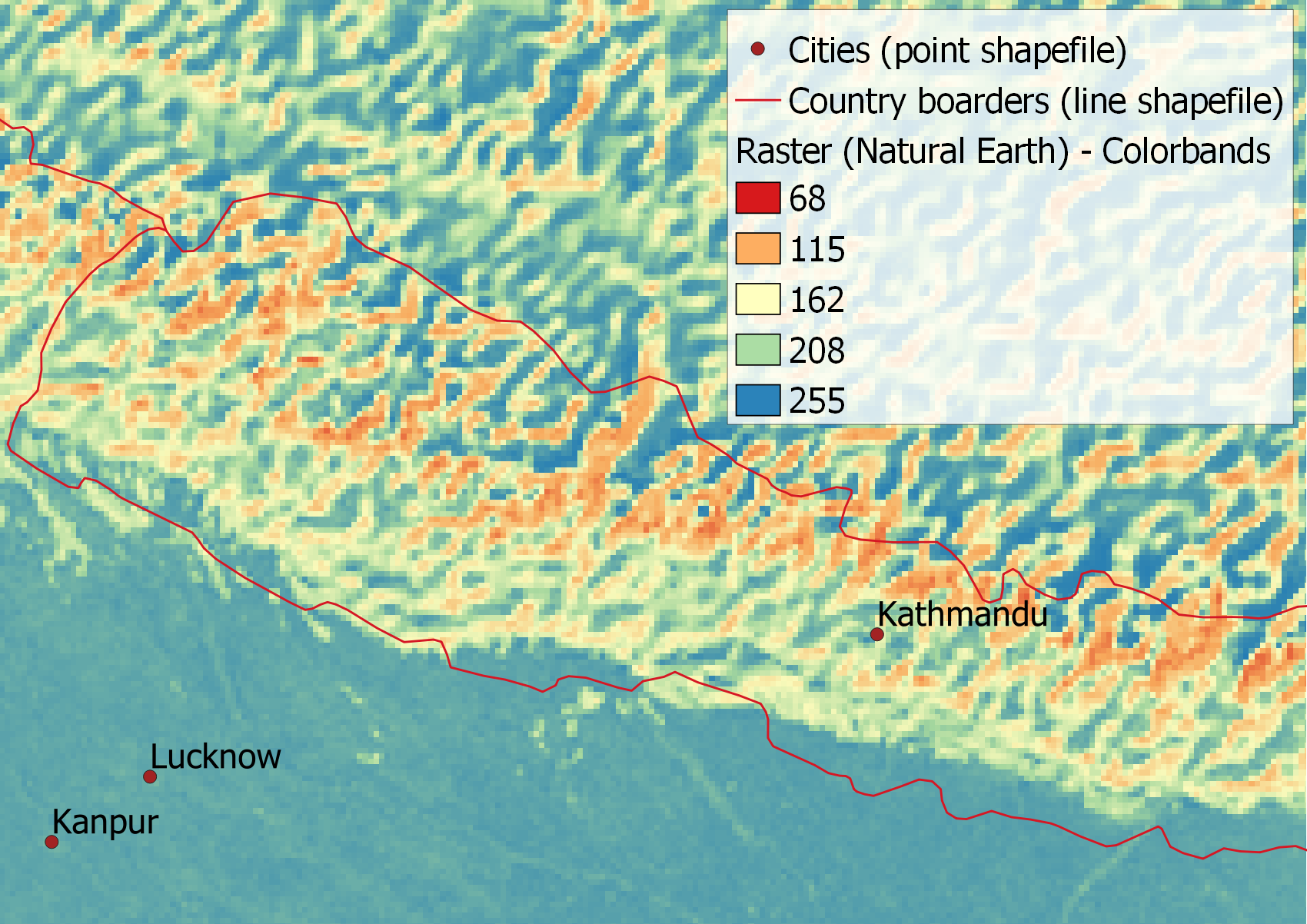
Illustration des NE1 50M SR W.tif-Rasters der natürlichen Erde, das auf Nepal gezoomt wurde, mit Punkt- und Linienformdateien, die auf Großstädte bzw. Ländergrenzen hinweisen. Beachten Sie das kachelartige Erscheinungsbild des Gitters, bei dem jede Kachel einer 50m-x-50m-Rasterzelle entspricht.
Lidar und Unterwasser Digitale Höhenmodelle (Bathymetrien)¶
Terrain survey data are often delivered in the shape of an x-y-z point dataset along with point attribute parameters. Three-dimensional datasets of the bare Earth’s topographic surface are referred to as a Digital Elevation Model (read more about Digitales Oberflächenmodell terminology in the glossary), which represents the baseline for any physical analysis of a river ecosystem. The underwater topography is called the bathymetry of a river or other water body. Nowadays, x-y-z point clouds for generating a DEM mostly stem from Lidar combined with Echolot surveys. Older approaches rely on manual surveying (e.g., with a total station) of cross-sectional river profiles and interpolating the terrain between the profiles. The newer Lidar technique employs light (laser) sources and provides bathymetry data up to 2-m deep water in the form of *.las or the zipped form *.laz files. Deeper waters are mapped with an Echolot and the merged Lidar and echo-sounding datasets produce seamless point clouds of river ecosystems, which may be stored in different file types.
Lidar produces massive point clouds, which quickly overcharge even powerful computers. This is why in practice, Lidar data may need to be broken down into smaller zones of less than 106 points each. Particular Lidar processing software (e.g., LAStools) is helpful in this task.
Projektionen und Koordinatensysteme¶
In geospatial data analyses, a projection represents an approach to flatten (a part of) the globe. In this flattening process, latitudinal (North/South) and longitudinal (West/East) coordinates of a location on the globe (three-dimensional - 3d) are projected onto the coordinates of a two-dimensional (2d) map. When 3d coordinates are projected onto 2d coordinates, distortions occur, and a variety of projection systems are used in geospatial analyses. In practice, this means that if we use geospatial data files with different projections, a distortion effect propagates into all subsequent calculations. It is crucial to avoid such distortion effects by ensuring that the same projection and coordinate reference system (CRS) is applied consistently to all geospatial data. This starts with the creation of a new geospatial layer (e.g., a point vector shapefile or GeoPackage) in QGIS (get installation instructions) and should be used consistently in all program codes. To specify a CRS; for instance, in QGIS (tutorial in the next section), click on Project > Properties > CRS tab and select a COORDINATE_SYSTEM. For example, an appropriate coordinate system for central Europe is ESRI:31493 (read more in the QGIS docs). Projected systems vary with region (local coordinate systems), which can be found, for example, at epsg.io or spatialreference
In shapefiles, information about the projection is stored in a .prj file (recall definitions in the shapefile section), which is a plain text file. The Open Geospatial Consortium (OGC) and Esri use Well-Known Text (WKT) files for standard descriptions of coordinate systems, and a WKT-formatted .prj file is shown in the code block below. The units and measures defined in the WKT-formatted .prj file also determine the units of WKB (Well-Known Binary) definitions of geometries such as line length (e.g., in meters, feet, or many more), or polygon area (square meters, square kilometers, acres, and many more).
PROJCS["unknown",GEOGCS["GCS_unknown",
                        DATUM["D_Unknown_based_on_GRS80_ellipsoid",SPHEROID["GRS_1980",6378137.0,298.257222101]],
                        PRIMEM["Greenwich",0.0],UNIT["Degree",0.0174532925199433]],
       PROJECTION["Lambert_Conformal_Conic"], PARAMETER["False_Easting",6561666.66666667],
       ..., UNIT["US survey foot",0.304800609601219]]
In GeoJSON files, the default coordinate reference system is WGS 84 (longitude/latitude, EPSG:4326), as mandated by RFC 7946 §4.