Basic (Text) Dateihandling, NumPy, pandas und DateTime.
Run this notebook in your web browser: 
Der Link öffnet b06-pynum.py als interaktives marimo Notebook, das vollständig in Ihrem Webbrowser läuft, ohne etwas zu installieren.
Warten Sie einen Moment, bis Python im Browser geladen ist (das dauert nur am ersten Start länger).
Klicken Sie auf die gelbe Starttaste (▶, unten rechts) um alle Zellen auszuführen.
Bearbeiten und re-run jede Codezelle zu experimentieren: marimo automatisch aktualisiert alle Zellen, die davon abhängig sind.
Ihre Bearbeitungen bleiben nur im Browser-Tab. Um sie zu halten, speichern Sie das Notizbuch durch das Menü (≠, oben rechts) > Export... > Python.
Run this marimo notebook locally
Um b06-pynum.py auf Ihrem eigenen Gerät zu betreiben, erhalten Sie es vom marimo
Repository:
git clone https://github.com/sschwindt/marimo-python-course.gitDie Kursumgebung erstellen und aktivieren:
conda env create -f environment.ymlundconda activate hy-marimoStarten Sie im Ordner Repository das Notebook mit
marimo edit b06-pynum.py
Run this notebook with Jupyter
This page is also available as the Jupyter notebook b06-pynum.ipynb in the jupyter , or install Python and JupyterLab locally to run b06-pynum.ipynb on your own machine.
Watch this section in video format
Watch this section as a video on the @hydroinformatics channel on YouTube.
Laden und Schreiben von grundlegenden Datendateien
Data can be stored in many different (text) file formats such as txt or csv files. Python provides the open(file) and write(...) functions to read and write data from nearly every text file format. In addition, there are packages such as csv (for csv files), which simplify handling specific file types. The following sections illustrate the use of the open(file) and write(...) functions. The later shown pandas module provides more functions to import and export numeric data along with row and column headers.
Textdateidaten laden (open)
Der Befehl open lädt Textdateien als Dateiobjekt in Python. Die Syntax des Befehls open lautet:
open("file-name", "mode")wobei:
file-nameis the file to open (e.g.,"data.txt"); if the file is not in the script directory, the filename needs to be extended by the full directory (path) to the data file (e.g.,"C:/experiment1/data.txt").modedefines the access type and it can take the following values:"r"- schreibgeschützt (Standardwert, wenn kein"mode"-Wert angegeben ist); die Datei kann nicht geändert oder überschrieben werden."rb"- schreibgeschützt im Binärformat; das Binärformat ist vorteilhaft, wenn die Datei keine Textdatei ist, sondern Medien wie Bilder oder Videos."r+"- lesen und schreiben."w"- Write-only; eine neue Datei wird erstellt, wenn eine Datei mit dem bereitgestelltenfile-namenoch nicht existiert."wb"- Schreibe nur im Binärmodus."w+"- erstellen, schreiben und lesen."wb+"- schreiben und lesen Sie im Binärmodus."a"- neue Daten an eine Datei anhängen; der Schreibzeiger wird am Ende der Datei platziert und eine neue Datei erstellt, wenn eine Datei mit dem bereitgestelltenfile namenoch nicht existiert."ab"- neue Daten im Binärmodus anhängen."a+"- both append (write at the end) and read."ab+"- Anfügen und Lesen von Daten im Binärmodus.
When "r" or "w" modes are used, the file pointer (i.e, the blinking cursor that you can see, for example, in Word documents) is placed at the beginning of the file. For "a" modes, the file pointer is placed at the end of the file.
It is good practice to read and write data from and to a file within a with statement to avoid file lock issues. For example, the following code block creates a new text file within a with statement:
with open("data/new.csv", mode="w+") as file:
file.write("And yet it moves.")Read-only
Once the file object is created, we can parse the file and copy the file data content to a desired Python data type (e.g., a list, tuple or dictionary). Parsing the data works with for-loops (other loop types will also work) to iterate on lines and line entries. The lines represent strings and data columns can be separated by using the built-in string function line_as_list = str().split("SEPARATOR"), where "SEPARATOR" can be "," (comma), ";" (semicolon), "\t" (tab), or any other sign. After reading all data from a file, use file_object.close() to avoid that the file is locked by Python and cannot be opened by another program.
The following example opens a text file called pure-numbers.txt (download pure-numbers.txt into a local sub-folder called data) that contains float numbers between 0.0 and 10.0. The file has 17 data rows (e.g., for 17 experimental runs) and 4 data columns (e.g., for 4 measurements per experimental run), which are separated by a TAB ("\t" separator). The below code block uses the built-in function readlines() to parse the file lines, splits the lines using the "\t" separator, and loops over the line entries to append them to the list variable data_list only if entry is numeric (verified with the try - except statement). data_list is a nested list that is initiated at the beginning of the script and a sub-list (nested list) is appended for every file line (row).
file_object = open("data/pure-numbers.txt")  # read file with default "mode"="r"

data_list = []  # this will be a nested list with 17 sub-lists (rows) containing 4 entries (columns)=

for line in file_object.readlines():
    line_as_list = line.split("\t")  # converts the line into a list using a tab (\t) separator
    data_list.append([])  # append an empty sub-list for every file line (17 rows)
    for entry in line_as_list:
        try:
            # try to append the entry as floating point number to the last sub-list, which is pointed at using [-1]
            data_list[-1].append(float(entry))
        except ValueError:
            # if entry is not numeric, append 0.0 to the sub-list and print a warning message
            print("Warning: %s is not a number. Replacing value with 0.0." % str(entry))

# verify that data_list contains the 17 rows (sub-lists) with the built-in list function __len__()
print("Number of rows: %d" % len(data_list))

# verify that the first sub-list has four entries (number of columns)
print("Number of columns: %d" % len(data_list[0]))

file_object.close()  # close file (otherwise it will be locked as long as Python is still running!) alternative: use with-statement
print(data_list)  # print the data
Number of rows: 17
Number of columns: 4
[[2.202, 3.658, 0.201, 1.651], [0.904, 0.643, 1.094, 1.859], [2.104, 2.786, 2.212, 3.489], [1.181, 4.415, 0.331, 3.418], [2.203, 2.882, 0.874, 1.151], [4.044, 4.848, 1.704, 3.523], [4.407, 4.494, 0.608, 0.387], [1.015, 4.415, 0.672, 2.221], [4.798, 2.759, 3.521, 1.714], [3.495, 4.206, 0.288, 3.801], [4.947, 3.791, 1.546, 3.989], [0.695, 2.35, 4.561, 1.609], [1.581, 0.824, 0.293, 3.458], [1.216, 1.475, 2.56, 0.456], [2.956, 0.904, 3.029, 3.559], [0.691, 2.187, 3.533, 2.188], [0.44, 2.772, 3.386, 2.671]]
Erstellen und Schreiben von Dateien
A file is created with the "w" or "a" modes (e.g., open(file_name, mode="a")).
Imagine that the loaded data_list contains measurements in mm. For each value in each sub-list, append the string "nan" to new_data_list if the value is less than or equal to 1.0; otherwise, preserve the original numeric value. If indices are used explicitly, access a nested-list value as data_list[i][j].
Use a with statement and context manager to ensure that the file is closed automatically after the block finishes.
# create a new list and overwrite all values <= 1.0 with nan
new_data_list = []
for i in data_list:
    new_data_list.append([])
    for j in i:
        if j <= 1.0:
            new_data_list[-1].append("nan")
        else:
            new_data_list[-1].append(j)

print(new_data_list)
# write the modified new_data_list to a new text file
new_file = open("data/modified-data.csv", mode="w+")  # lets just use csv: Python does not care about the file ending (could also be file.wayne)
for row in new_data_list:
    new_line = ", ".join([str(e) for e in row]) + "\n"
    new_file.write(new_line)
new_file.close()
[[2.202, 3.658, 'nan', 1.651], ['nan', 'nan', 1.094, 1.859], [2.104, 2.786, 2.212, 3.489], [1.181, 4.415, 'nan', 3.418], [2.203, 2.882, 'nan', 1.151], [4.044, 4.848, 1.704, 3.523], [4.407, 4.494, 'nan', 'nan'], [1.015, 4.415, 'nan', 2.221], [4.798, 2.759, 3.521, 1.714], [3.495, 4.206, 'nan', 3.801], [4.947, 3.791, 1.546, 3.989], ['nan', 2.35, 4.561, 1.609], [1.581, 'nan', 'nan', 3.458], [1.216, 1.475, 2.56, 'nan'], [2.956, 'nan', 3.029, 3.559], ['nan', 2.187, 3.533, 2.188], ['nan', 2.772, 3.386, 2.671]]
Ändern bestehender Dateien
Existing text files can be opened and modified in either mode="r+" (pretending that information needs to be read before it is modified) or mode="a+". Recall that "r+" will place the pointer at the beginning of the file and "a+" will place the pointer at the end of the file. Thus, if we want to modify lines or entries of an existing file, "r+" is the good choice and if we want to append data at the end of the file, "a" is the good choice (+ is not strictly needed in the case of "a"). This section shows two examples: (1) modification of existing data in a file using "r+", and (2) appending data to an existing file using "a".
- Example 1 - Replace data in an existing file with
"r+" In the previous code block, we eliminated all measurements that were smaller than 1 mm because of the precision of the measurement device. However, we have retained all other values with two-digit accuracy - an accuracy that is not given. Consequently, all decimal places in the measurements must also be eliminated. To achieve this, we have to round all measured values with Python’s built-in round function (
round(number, n-digits)) to zero decimal places (i.e.,n-digits = 0). In this example (featured in the below code block), an exceptionIOErroris raised when the file"data/modified-data.csv"does not exist (or if it is locked by another software). Anifstatement ensures that rounding the data is only attempted if the file exists. The overwriting procedure first reads all lines of the file into thelinesvariable. After reading all lines, the pointer is at the end of the file, andfile.seek(0)puts the pointer back to position 0 (i.e., at the beginning of the file).file.truncate()purges the file. Thus, the original file is blank for a moment and all file contents are stored in thelinesvariable. Rounding the data happens within a for-loop that:Splits the comma-separated line string (produces
lines_as_list).Creates the temporary list
_numeric_line_, where rounded, numeric values are stored (the variable is overwritten in every iteration).Schleifen über die Zeileneinträge (
line_as_list), wobei eine Ausnahmeanweisung gerundet (auf Nullstellen), numerische Werte und"nan"anhängt, wenn ein Eintrag nicht numerisch ist.Writes the modified line to the
"data/modified-data.csv"csv file.
Finally, the csv is closed with
modified_file.close().
try:
  with open("data/modified-data.csv", mode="r+") as modified_file:
	  lines = modified_file.readlines()
	  modified_file.seek(0)
	  modified_file.truncate()

	  for line in lines:
		  line_as_list = line.split(", ")
		  numeric_line = []
		  for entry in line_as_list:
			  try:
				  numeric_line.append(round(float(entry), 0))
			  except ValueError:
				  numeric_line.append(entry.strip())
		  modified_file.write(", ".join(str(entry) for entry in numeric_line) + "\n")
  print("Processed file.")
except OSError as error:
  print(f"Could not process the file: {error}")
Processed file.
Theoretisch kann der obige Code-Snippet als Funktion umgeschrieben werden, um beliebige Daten in einer Datei zu ändern. Darüber hinaus können andere Schwellenwerte oder bestimmte Datenbereiche mit if - else-Anweisungen gefiltert werden.
- Example 2 - Append data to an existing file with
"a+" By coincidence, you find a hand-written measurement protocol that has data of an 18th experimental run, which is not in the electronic measurement data file due to a data transmission error. Now, you want to add the data to the above-produced csv file. Entering the data does not take much work, because only 4 measurements were performed per experimental run and the below code block contains the hand-written data in a list variable called
forgotten_data. This example uses theosmodule (recall Pakete, Module und Bibliotheken) to verify if the data file exists withos.path.isfile()(theos.getcwd()statement is a gadget here). The code block features the usage of awithstatement (i.e., awith- context manager or name space).The essential part of the code that writes the line to the data file is
file.write(line), wherelinecorresponds to the above-introduced", ".join(list-of-strings) + "\n"string.
import os
print(os.getcwd())
forgotten_data = [4.0, 3.0, "nan", 8.0]

if os.path.isfile("data/modified-data.csv"):
    with open("data/modified-data.csv", mode="a") as file_object:
        file_object.write(", ".join([str(e) for e in forgotten_data]) + "\n")
    print("Data appended.")
else:
    print("The file does not exist.")
/home/schwindt/github/hyhome-v2/jupyter
Data appended.
NumPy
NumPy bietet hochrangige mathematische Funktionen für lineare Algebra, einschließlich Operationen auf mehrdimensionalen Arrays und Matrizen. Die Open-Source-Bibliothek NumPy (für Numerical Python) ist in Python und [C](C (programming language)] geschrieben und enthält eine umfassende Dokumentation (die neueste Version auf der Website des Entwicklers herunterladen oder lesen Sie das Online-Tutorial des Entwicklers].)
Watch the NumPy section in video format
Watch this section as a video on the @hydroinformatics channel on YouTube.
Installation
NumPy kann über Anaconda (recall instructions) installiert werden und die Entwickler empfehlen die Verwendung einer wissenschaftlichen Python-Distribution (Anaconda) mit SciPy Stack].
The provided Anaconda environment.yml (flussenv) already includes NumPy (more information in the installation section). Similarly, Linux users will have NumPy installed in a virtual environment (e.g., vflussenv) with pip (recall pip-installing flusstools). Otherwise, to install NumPy in any other conda environment, open Anaconda Prompt (Start > type Anaconda Prompt) and type:
conda activate ENVIRONMENT-NAME
conda install numpy
Um NumPy in einer anderen virtuellen Umgebung zu installieren, tippen Sie auf:
pip install numpyNutzung
The NumPy library is typically imported with import numpy as np. Create a NumPy array with np.array(values), where values is array-like input such as a list or tuple. Nested sequences can be used to create multidimensional arrays; for example, np.array([[1, 2, 3], [4, 5, 6]]) creates an array with two rows and three columns.
The following code block shows very basic usage of NumPy (or: numpy) imported as np and the creation of a 2x3 numpy array. The rounded parentheses indicated that the value sequence of the np.array represents a tuple for creating a multi-dimensional array.
import numpy as np
an_array = np.array(([2, 3, 1], [4, 5, 6]))
print(an_array)
[[2 3 1]
[4 5 6]]
NumPy-Arrays (Datentyp: ndarray) haben viele eingebaute Funktionen, z. B. um die Arraygröße auszugeben:
print(type(an_array))
print("Array dimensions: " + str(an_array.shape))
print("Total number of array elements: " + str(an_array.size))
print("Number of array axes: " + str(an_array.ndim))
<class 'numpy.ndarray'>
Array dimensions: (2, 3)
Total number of array elements: 6
Number of array axes: 2
There are many types of np.arrays and many ways to create them:
print(np.array([(2, 3, 1), (4, 5, 6)]))  # the same as an_array
print(np.array([[2, 3, 1], [4, 5, 6]], dtype=complex))
[[2 3 1]
[4 5 6]]
[[2.+0.j 3.+0.j 1.+0.j]
[4.+0.j 5.+0.j 6.+0.j]]
Arrays von Nullen oder Einsen oder leeren Arrays können mit * Integer * oder * Float * Datentypen erstellt werden. Beachten Sie bei der Erstellung solcher Arrays die Verwendung von Tupeln (dh Sequenzen, die mit abgerundeten Klammern umfasst sind), um Arraydimensionen zu definieren:
print(np.zeros((2,6)))
print(np.ones((2,6), dtype=np.float64))  # other dtypes: int16, np.int16, float, np.float32, np.complex64
print(np.empty((2,6)))
print(np.empty((2,6), dtype=np.int16))
[[0. 0. 0. 0. 0. 0.]
[0. 0. 0. 0. 0. 0.]]
[[1. 1. 1. 1. 1. 1.]
[1. 1. 1. 1. 1. 1.]]
[[1. 1. 1. 1. 1. 1.]
[1. 1. 1. 1. 1. 1.]]
[[19880 11437 6 0 0 0]
[ 0 0 0 0 0 0]]
np.empty(shape) allocates an array without initializing its entries. Any displayed values are arbitrary remnants of memory and may differ between runs. Fill every entry before reading or using the array; use np.zeros(shape) or np.ones(shape) when initialized values are required.
NumPy stellt die Funktion arange(start, end, step-size) zur Verfügung, um numerische Sequenzen zu erstellen. Solche Sequenzen repräsentieren Arrays (ndarray), die später umgeformt werden können (d.h. in Spalten und Zeilen neu organisiert).
print("1D array:")
print(np.arange(0, 10, 2))  # 1D array
print("\n2D array:")
print(np.arange(0, 12, 2).reshape(2, 3))  # 2D array
print("\n3D array:")
print(np.arange(1, 13, 1).reshape(2, 2, 3))  # 3D array
print("\n1D Linspace (start, end, number-of-elements):")
print(np.linspace(0, np.pi, 3))
1D array:
[0 2 4 6 8]
2D array:
[[ 0 2 4]
[ 6 8 10]]
3D array:
[[[ 1 2 3]
[ 4 5 6]]
[[ 7 8 9]
[10 11 12]]]
1D Linspace (start, end, number-of-elements):
[0. 1.57079633 3.14159265]
Random numbers can be generated with NumPy’s random number generator np.random and its .random(range_tuple) function.
rand_array = np.random.random((2,4))
print(rand_array)
[[0.78599116 0.11777177 0.29913723 0.9290063 ]
[0.70878365 0.5521523 0.81552564 0.17867719]]
Integrierte Array-Funktionen ermöglichen es, minimale oder maximale Werte oder Summen von Arrays zu finden:
print("Sum of 12-elements ones-array: " + str(np.ones((2,6)).sum()))
print("Minimum: " + str(an_array.min()))
print("Maximum: " + str(an_array.max()))
Sum of 12-elements ones-array: 12.0
Minimum: 1
Maximum: 6
Farbfelder
Arrays may also contain color information, where colors represent a mix of the three base colors red, green, and blue (RGB). Thus, one color can be defined as [red-value, green-value, blue-value], and a value of 0 means that a color tone is not present, while 255 is its maximum value. There is no color when all color tone values are zero, which corresponds to black; when all color tones are maximum (255), the color mix corresponds to white. This way, array elements can be lists of color tones, and plotting such arrays produces images. The following example produces an array with 5 color-list elements, which could be plotted as a very basic image with 5 pixels (one black, red, green, blue, and white, respectively):
color_set = np.array([[0, 0, 0],         # black
                      [255, 0, 0],       # red
                      [0, 255, 0],       # green
                      [0, 0, 255],       # blue
                      [255, 255, 255]])  # white
Array (Matrix)
Array-Berechnungen (Matrix-Operationen) folgen den Regeln der linearen Algebra:
A = np.random.random((2,4))
B = np.random.random((4,2))
print("Subtraction: " + str(A.transpose() - B))
print("Element-wise product: " + str(A.transpose() * B))
print("Matrix product (option 1): " + str(A @ B))
print("Matrix product (option 2): " + str(A.dot(B)))
Subtraction: [[ 0.39513798 0.92256882]
[ 0.34627686 -0.64066838]
[-0.41525172 0.49672182]
[-0.64648598 0.21224637]]
Element-wise product: [[0.02631898 0.05370238]
[0.2312502 0.07207233]
[0.28977301 0.14078519]
[0.10386917 0.18425933]]
Matrix product (option 1): [[0.65121136 0.64929413]
[1.06516605 0.45081924]]
Matrix product (option 2): [[0.65121136 0.64929413]
[1.06516605 0.45081924]]
Weitere elementweise Berechnungen umfassen exponentiell (**), geometrisch (np.sin, np.cos, np.tan, etc.) und boolesche Operatoren:
print("A to the power of 3: " + str(A**3))
print("Exponential: " + str(np.exp(A)))
print("Square root: " + str(np.sqrt(A)))
print("Sine of A times 3: " + str(np.sin(A) * 3))
print("Boolean where A is smaller than 0.3: " + str(A < 0.3))
A to the power of 3: [[9.30892075e-02 3.20353634e-01 5.03795493e-02 2.36414082e-03]
[9.34027227e-01 9.30307166e-04 3.40544706e-01 1.64838161e-01]]
Exponential: [[1.57335504 1.9822692 1.44676927 1.14249724]
[2.65782184 1.10254456 2.01038396 1.73031119]]
Square root: [[0.67320896 0.82718937 0.60772772 0.36498826]
[0.9886895 0.31244319 0.83565886 0.74047368]]
Sine of A times 3: [[1.313562 1.89625803 1.08298042 0.39846826]
[2.48731829 0.29239731 1.9288087 1.56371481]]
Boolean where A is smaller than 0.3: [[False False False True]
[False True False False]]
Array Form Manipulation
Manchmal ist es notwendig, ein mehrdimensionales Array in einen Vektor zu stapeln oder die Form eines Arrays neu zu gestalten. Neben der reshape()-Funktion gibt es noch einige weitere Optionen, um die Form eines Arrays zu manipulieren:
print("Flattened matrix A (into a vector):\n" + str(A.ravel()))
print("\nTranspose matrix A and append B:\n" + str(np.array([A.transpose(), B])))
print("\nTranspose matrix A and append B and cast into a (4x4) array:\n" + str(np.array([A.transpose(), B]).reshape(4,4)))
Flattened matrix A (into a vector):
[0.45321031 0.68424225 0.36933298 0.13321643 0.97750693 0.09762075
0.69832573 0.54830127]
Transpose matrix A and append B:
[[[0.45321031 0.97750693]
[0.68424225 0.09762075]
[0.36933298 0.69832573]
[0.13321643 0.54830127]]
[[0.05807233 0.05493811]
[0.33796539 0.73828912]
[0.78458471 0.20160391]
[0.77970241 0.33605491]]]
Transpose matrix A and append B and cast into a (4x4) array:
[[0.45321031 0.97750693 0.68424225 0.09762075]
[0.36933298 0.69832573 0.13321643 0.54830127]
[0.05807233 0.05493811 0.33796539 0.73828912]
[0.78458471 0.20160391 0.77970241 0.33605491]]
NumPy Dateihandling und np.nan
In the above examples on file handling, measurement data were loaded from text files, manipulated (modified), and (re-)written. The data manipulation involved the introduction of "nan" (not-a-number) values, which were excluded because measurements <1 mm were considered errors. Why didn’t we use zeros here? Zeros are numbers, too, and have a significant effect on data statistics (e.g., for calculating mean values). However, the "nan" string value may cause difficulties in data handling, in particular regarding the consistency of function output. NumPy provides with the np.nan data type a powerful alternative to the tedious "nan" string.
NumPy also has a text file load function called np.loadtxt(file-name, *args, **kwargs), which imports text files as np.arrays of float values. The default float value type can be adapted with the optional keyword dtype. Other optional keyword arguments are:
delimiter=STR(z. B.delimiter=';'), wobei der Standard"None"ist.usecols=TUPLE(z. B.usecols=(1, 3)extrahiert die Spalte 2nd und 4th), wobei auch ein * ganzzahliger* Wert nur in einer Spalte gelesen werden kannskiprows=INT(z. B.skiprows=2überspringt die ersten beiden Zeilen), wobei der Standard0ist.Weitere Argumente sind verfügbar und unter NumPy documentation aufgeführt.
Im folgenden Beispiel wird die oben erstellte csv-Datei data/modified-data.csv mit integer und "nan" string-Werten geladen, die automatisch in np.nan konvertiert werden.
experiment_data = np.loadtxt("data/modified-data.csv", delimiter=",")
print("This is the data 4th line (row): " + str(experiment_data[3, :]))
print("The data type of the 3rd (%s) entry is: " % str(experiment_data[3, 2]) + str(type(experiment_data[3, 2])))
This is the data 4th line (row): [ 1. 4. nan 3.]
The data type of the 3rd (nan) entry is: <class 'numpy.float64'>
Zusätzlich oder alternativ nimmt die Funktion np.load() Daten aus dateiähnlichen .npz, .npy oder gepickelten (gespeicherten Python-Objekten) Datenquellen auf (weitere Informationen finden Sie unter NumPy docs].
Statistik
The above examples featured array functions to assess basic array statistics such as the minimum and maximum. NumPy provides many more functions for array statistics such as the mean, median, or standard deviation, including functions that account for np.nan values. The following example illustrates some of the statistical functions with the experimental data from the above examples. Note the usage of nanmean instead of mean and statistics along array axis, where the optional keyword argument axis=0 corresponds to columns and axis=1 to statistics along rows in 2-dimensional arrays (maximum axis number corresponds to the array dimensions n minus 1, i.e., maximum axis=n-1).
print("Mean value (without nan): " + str(np.mean(experiment_data)))  # no applicable result
print("Mean value with np.nan: " + str(np.nanmean(experiment_data)))
print("Mean value along axis 0 (columns): " + str(np.nanmean(experiment_data, axis=0)))
print("Mean value along axis 1 (rows): " + str(np.nanmean(experiment_data, axis=1)))
Mean value (without nan): nan
Mean value with np.nan: 3.018181818181818
Mean value along axis 0 (columns): [2.78571429 3.26666667 2.9 3.0625 ]
Mean value along axis 1 (rows): [2.66666667 1.5 2.5 2.66666667 2. 3.75
4. 2.33333333 3.5 3.66666667 3.75 3.
2.5 1.66666667 3.33333333 2.66666667 3. 5. ]
Die folgenden Absätze stellen eine tabellarische Übersicht der statistischen Funktionen in NumPy dar (Quelle: NumPy docs). Die aufgeführten Funktionen stellen nur die Baseline dar und NumPy bietet viele weitere Optionen, die mit einer beliebigen Suchmaschine mit NumPy und der gewünschten Funktion als Suchschlüsselwort genutzt werden können.
Statistische Grundfunktionen
| Function | Description |
|---|---|
nanmin(a[, axis, out, keepdims]) | Minimum of an array or along an axis, ignoring np.nan. |
nanmax(a[, axis, out, keepdims]) | Maximum of an array or along an axis, ignoring np.nan. |
ptp(a[, axis, out]) | Range of values (max - min) along an axis. |
percentile(a, q[, axis, out, ...]) | q-th percentile of data along a specified axis. |
nanpercentile(a, q[, axis, out, ...]) | q-th percentile of data along a specified axis, ignoring np.nan. |
Mittelwert (Mittelwert), Standardabweichung und Varianzen
| Function | Description |
|---|---|
median(a[, axis, out, overwrite_input, keepdims]) | Median along an (optional) axis. |
average(a[, axis, weights, returned]) | Weighted average along an (optional) axis. |
mean(a[, axis, dtype, out, keepdims]) | Arithmetic mean along an (optional) axis. |
std(a[, axis, dtype, out, ddof, keepdims]) | Standard deviation along an (optional) axis. |
var(a[, axis, dtype, out, ddof, keepdims]) | Variance along an (optional) axis. |
nanmedian(a[, axis, out, overwrite_input, ...]) | Median along an (optional) axis, ignoring np.nan. |
nanmean(a[, axis, dtype, out, keepdims]) | Arithmetic mean along an (optional) axis, ignoring np.nan. |
nanstd(a[, axis, dtype, out, ddof, keepdims]) | Standard deviation along an (optional) axis, while ignoring np.nan. |
Korrelierende Daten (Arrays)
| Function | Description |
|---|---|
corrcoef(x[, y, rowvar, bias, ddof]) | Pearson (product-moment) correlation coefficients. |
correlate(a, v[, mode]) | Cross-correlation of two 1-dimensional sequences. |
cov(m[, y, rowvar, bias, ddof, fweights, ...]) | Estimate covariance matrix, based on data and weights. |
Histogramme erzeugen und zeichnen
| Function | Description |
|---|---|
histogram(a[, bins, range, normed, weights, ...]) | Histogram of a set of data. |
histogram2d(x, y[, bins, range, normed, weights]) | Bi-dimensional histogram of two data samples. |
histogramdd(sample[, bins, range, normed, ...]) | Multidimensional histogram of some data. |
bincount(x[, weights, minlength]) | Count number of occurrences of each value in array of non-negative ints. |
digitize(x, bins[, right]) | Indices of the bins to which each value in input array belongs. |
Kann *NumPy * *MATLAB * & reg;?
Erwägen Sie den Wechsel zu Python, nachdem Sie sanft mit * MATLAB®*-ähnlicher Software begonnen haben? Es gibt viele Gründe, Datenanalysen mit Python zu verbessern, und hier sind einige Moderatoren für frühere * MATLAB & reg; * Benutzer:
MATLAB® matrices can be loaded and saved with
scipy.io.loadmat(matrix-file-name)(useimport scipy).NumPys
np.arrayersetzt *MATLAB®*s Matrixnotation (obwohl es den historischen, veralteten NumPy Datentypnp.matrixgibt).Importieren Sie viele MATLAB®-Funktionen von
np.matlib(z. B.from numpy.matlib import rand, zeros, ones, empty, eye)oder allgemeinerimport numpy.matlib as M).Finden Sie das NumPy Äquivalent von vielen MATLAB® Funktion in der NumPy documentation].
Um die Plot-Funktionen von MATLAB® zu emulieren, verwenden Sie das
pylab-Paket und importieren es alsfrom pylab import *.
⚠ Dies überschreibt alle anderen (Standard-) Definitionen derplot()-Funktion undarray()-Objekte. Diese Nutzung ist also veraltet. Lesen Sie den Plotabschnitt für umfassende Plotanweisungen mit Python.]
MATLAB® ist eine eingetragene Marke von The MathWorks.
Pandas
pandas ist eine leistungsstarke Bibliothek für Datenanalysen und -manipulation mit Python. Es kann NumPy-Arrays verarbeiten, und beide Pakete stellen gemeinsam eine leistungsstarke Datenverarbeitungsmaschine dar. Die Macht von pandas liegt in der Verarbeitung von Datenrahmen, Datenbeschriftung (z. B. arbeitsmappenähnliche Spaltennamen) und flexiblen Dateiverarbeitungsfunktionen (z. B. die eingebaute read_csv(csv-file)-Funktion). Während NumPy-Arrays Berechnungen mit mehrdimensionalen Arrays (über zweidimensionale Tabellen hinaus) und geringem Speicherverbrauch ermöglichen, verarbeiten und beschriften pandas DataFrames Tabellendaten effizient mit mehr als ~100.000 Zeilen. Aufgrund seiner Kennzeichnungskapazität findet pandas auch breite Anwendung im maschinellen Lernen. Zusammenfassend lässt sich sagen, dass die Funktionalität von pandas auf NumPy aufbaut und beide Bibliotheken von der SciPy (Scientific Computing Tools for Python)-Community verwaltet werden, die auch matplotlib (siehe plotting section) und IPython (Jupyters Python-Kernel) produziert.
Watch the pandas section on YouTube
Watch this section as a video on the @hydroinformatics channel on YouTube.
Installation
pandas kann über Anaconda (recall instructions) installiert werden und die Entwickler empfehlen die Verwendung einer wissenschaftlichen Python-Distribution (Anaconda) mit SciPy Stack].
Die bereitgestellte Anaconda environment.yml (flussenv) enthält bereits pandas (weitere Informationen im installation-Bereich). Ebenso werden Linux-Benutzer pandas in einer virtuellen Umgebung (z. B. vflussenv) mit pip installiert haben (rufen Sie pip-installing flusstools zurück). Andernfalls, um pandas in einer anderen conda-Umgebung zu installieren, öffnen Sie Anaconda Prompt (Start > Typ Anaconda Prompt) und geben Sie:
conda activate ENVIRONMENT-NAME
conda install pandas
Um pandas in einer anderen virtuellen Umgebung zu installieren, tippen Sie auf:
pip install pandasNutzung
pandas standard import alias ist pd: import pandas as pd. Die folgenden Abschnitte geben einen Überblick über grundlegende pandas-Funktionen und viele weitere Funktionen sind im Entwickler docs] dokumentiert.
Datenrahmen & Serie
The below code block illustrates one way to create a pandas data frame (pd.DataFrame), one of pandas core objects. Note the difference between a 1-dimensional series pd.Series (corresponds to a one-column data frame), and an n-dimensional data frame with row (=index) and column names. The default row names number rows starting from 0 (unlike Office software that starts at row no. 1), without column names. Column names can be initially defined as a list and replaced with a dictionary that maps the initial list entries to new names.
import pandas as pd

print("A 1-column pd.DataFrame:\n"+ str(pd.Series([3, 4, np.nan])))  # a simple pandas data frame with one column

row_names = np.arange(1, 4, 1)
wb_like_df = pd.DataFrame(np.random.randn(len(row_names), 3),
                          index=row_names, columns=['A', 'B', 'C'])
print("\nThis is a workbook-like (row and column names) data frame:\n" + str(wb_like_df))
print("\nRename column names with dictionary:\n" + str(wb_like_df.rename(
        columns={'A': 'Series 1', 'B': 'Series 2', 'C': 'Series 3'})))
print("\nTranspose the data frame:\n" + str(wb_like_df.T))
A 1-column pd.DataFrame:
0 3.0
1 4.0
2 NaN
dtype: float64
This is a workbook-like (row and column names) data frame:
A B C
1 -0.374896 1.510560 0.164615
2 0.171686 -0.668994 -1.850155
3 -0.521211 1.688967 -0.653523
Rename column names with dictionary:
Series 1 Series 2 Series 3
1 -0.374896 1.510560 0.164615
2 0.171686 -0.668994 -1.850155
3 -0.521211 1.688967 -0.653523
Transpose the data frame:
1 2 3
A -0.374896 0.171686 -0.521211
B 1.510560 -0.668994 1.688967
C 0.164615 -1.850155 -0.653523
A pandas DataFrame object can also be created from a dictionary, where the dictionary keys define column names and the dictionary values constitute the data of every column:
df = pd.DataFrame({'Water depth': pd.Series(np.random.uniform(low=0.1, high=0.3, size=(4,)), dtype='float32'),
                   'Sediment': ["yes", "no", "yes", "no"],
                   'Flow regime': pd.Categorical(["fluvial", "fluvial", "supercritical", "critical"]),
                   'Water': "Always there"})
print("A dictionary-built data frame:\n" + str(df))
print("\nFrame data types:\n" + str(df.dtypes))
A dictionary-built data frame:
Water depth Sediment Flow regime Water
0 0.273525 yes fluvial Always there
1 0.168256 no fluvial Always there
2 0.297529 yes supercritical Always there
3 0.201709 no critical Always there
Frame data types:
Water depth float32
Sediment str
Flow regime category
Water str
dtype: object
Eingebaute Attribute und Methoden eines pandas DataFrame ermöglichen einen einfachen Zugriff auf den oberen (Kopf) und den unteren Teil eines Datenrahmens und viele weitere Objekteigenschaften (Rückruf: Verwenden Sie dir(dict_df) oder lesen Sie den docs des Entwicklers]):
print("Head of the dictionary-based dataframe (first two rows):\n" + str(df.head(2)))
print("\nEnd (tail) of the dictionary-based dataframe (last row):\n" + str(df.tail(1)))
Head of the dictionary-based dataframe (first two rows):
Water depth Sediment Flow regime Water
0 0.273525 yes fluvial Always there
1 0.168256 no fluvial Always there
End (tail) of the dictionary-based dataframe (last row):
Water depth Sediment Flow regime Water
3 0.201709 no critical Always there
Beispiel: Erstellen Sie eine pandas.DataFrame von Froude-Nummern
In hydraulics, the Froude-Zahl characterizes the flow regime as “fluvial” (Fr<1), “critical” (Fr=1), or “super-critical” (Fr>1). The precision of measurement devices in physical flume experiments makes the exact determination of the critical moment a challenge and forces researchers to apply an interval around 1, rather than the exact value of 1.0:
| Fr | (0.00, 0.95( | (0.95, 1.00( | (1.00) | )1.00, 1.05) | )1.05, inf( | |--------------------------------------------------------------------------------------------------------------------------------------------------------------------------------------------------------------------------------------------------------------- | Flow | fluvial | near-critical (langsam) | critical | near-critical (schnell) | super-critical |
pd.DataFrame( ... ) objects are a convenient way to classify and store flume experiment data:
def classify_froude(fr):
  if fr < 0.95:
	  return "fluvial"
  if fr < 1.0:
	  return "near-critical (slow)"
  if fr == 1.0:
	  return "critical"
  if fr <= 1.05:
	  return "near-critical (fast)"
  return "super-critical"

Fr_measured = np.random.uniform(low=0.01, high=2.00, size=10)
Fr_classified = [classify_froude(fr) for fr in Fr_measured]
obs_df = pd.DataFrame({"measured": Fr_measured, "flow regime": Fr_classified})
print(obs_df)
---------------------------------------------------------------------------
NameError                                 Traceback (most recent call last)
Cell In[1], line 12
      9 	  return "near-critical (fast)"
     10   return "super-critical"
---> 12 Fr_measured = np.random.uniform(low=0.01, high=2.00, size=10)
     13 Fr_classified = [classify_froude(fr) for fr in Fr_measured]
     14 obs_df = pd.DataFrame({"measured": Fr_measured, "flow regime": Fr_classified})

NameError: name 'np' is not defined
Daten an eine pandas.DataFrame
Avoid repeatedly inserting rows into a DataFrame. Collect new records first and construct a DataFrame once, or concatenate batches with pd.concat(). Assigning a complete column is direct and efficient.
Der folgende Codeblock veranschaulicht sowohl das Hinzufügen einer Zeile als auch einer Spalte zu einem vorhandenen *pandas * Datenrahmen.
import random

new_rows = pd.DataFrame({
  "measured": [0.996],
  "flow regime": ["near-critical (slow)"],
})
obs_df = pd.concat([obs_df, new_rows], ignore_index=True)
obs_df["with sediment"] = [bool(random.getrandbits(1)) for _ in range(len(obs_df))]
print(obs_df.tail(3))
    measured           flow regime  with sediment
8   1.541139        super-critical           True
9   0.189163               fluvial          False
10  0.996000  near-critical (slow)          False
NumPy Arrays und Pandas Datenrahmen
Ein NumPy-Array hat einen Datentyp (dtype), während ein Pandas DataFrame für jede Spalte einen anderen dtype verwenden kann. DataFrame.to_numpy() wählt einen gemeinsamen dtype für das resultierende Array aus und erfordert möglicherweise Typzwang oder eine Kopie, abhängig von den Spalten dtypes des DataFrame. DataFrame-Index- und Spaltenlabels sind im resultierenden Array nicht enthalten. Wenn eine Spalte der pandas DataFrame nicht numerisch ist, beinhaltet die Konvertierung das Kopieren des Objekts, was dann hohe Rechenkosten verursacht. Beachten Sie, dass die Bezeichnungen index und column eines pandas DataFrame bei der Konvertierung von pd.DataFrame zu np.ndarray verloren gehen.
print(obs_df.to_numpy())[[0.7228199423430681 'fluvial' True]
[1.0994432843154105 'super-critical' True]
[0.8865704358418128 'fluvial' False]
[0.8490886765821513 'fluvial' True]
[1.1750423214539258 'super-critical' True]
[0.086024140985809 'fluvial' True]
[1.1575177959070637 'super-critical' True]
[1.6067571441117197 'super-critical' False]
[1.5411388862372846 'super-critical' True]
[0.18916310404617928 'fluvial' False]
[0.996 'near-critical (slow)' False]]
Zugriff auf Datenrahmen Einträge
Elemente von Datenrahmen sind über das Spalten- und Zeilenlabel (df.loc[index=row, column-label]) oder die Nummer (df.iloc) zugänglich:
print("Label localization results in: " + str(df.loc[2, "Water depth"]))
print("Same result with integer grid location: " + str(df.iloc[2, 0]))
Label localization results in: 0.29752922
Same result with integer grid location: 0.29752922
Datenrahmen neu gestalten
Einzelne oder mehrere Zeilen (Indizes) und Spalten können aus neuen oder bestehenden DataFrame-Objekten extrahiert und kombiniert werden:
print(pd.DataFrame([df["Water depth"], df["Sediment"]])) 0 1 2 3
Water depth 0.273525 0.168256 0.297529 0.201709
Sediment yes no yes no
The df.stack() method pivots the columns of a data frame, which is a powerful tool to classify data that can take different dimensions (e.g., the volume and weight of 1 m3 water - read more about the stack method).
print(df.stack()[0])
df.unstack()  # unstack data frame
Water depth 0.273525
Sediment yes
Flow regime fluvial
Water Always there
dtype: object
Water depth  0         0.273525
             1         0.168256
             2         0.297529
             3         0.201709
Sediment     0              yes
             1               no
             2              yes
             3               no
Flow regime  0          fluvial
             1          fluvial
             2    supercritical
             3         critical
Water        0     Always there
             1     Always there
             2     Always there
             3     Always there
dtype: object
Big datasets often contain large amounts of data with many labels, but we are often only interested in a small subset of the data. To this end, data frame subsets can be created with df.pivot(index, columns, **values) (Pivot method):
print("Pivot table for \'Flow regime\':\n" + str(df.pivot(index="Sediment", columns="Water depth")["Flow regime"]))
print("\nPivot table for \'Water\':\n" + str(df.pivot(index="Sediment", columns="Water depth")["Water"]))
Pivot table for 'Flow regime':
Water depth 0.168256 0.201709 0.273525 0.297529
Sediment
no fluvial critical NaN NaN
yes NaN NaN fluvial supercritical
Pivot table for 'Water':
Water depth 0.168256 0.201709 0.273525 0.297529
Sediment
no Always there Always there NaN NaN
yes NaN NaN Always there Always there
Darüber hinaus ermöglicht df.pivot_table(index, columns, values, aggfunc) (Pivot table function]) eine inline Office-ähnliche Funktionsanwendung für eine oder mehrere Zeilen und/oder Spalten.
print("\'mean\' for \'Water depth\':\n" + str(df.pivot_table(index="Sediment", columns="Flow regime", values="Water depth", aggfunc=np.mean)))'mean' for 'Water depth':
Flow regime critical fluvial supercritical
Sediment
no 0.201709 0.168256 NaN
yes NaN 0.273525 0.297529
Lesen Sie mehr über das Umformen und Schwenken von Datenrahmen im Entwickler docs].
Dateihandling (csv, Arbeitsmappen und mehr)
*pandas * kann von vielen dateiendateitypen lesen und schreiben, was es extrem leistungsfähig für die analyse von daten macht. Die folgende Tabelle fasst die wichtigsten Dateitypen für numerische hydraulische, morphodynamische und fluviale Landschaftsanalysen zusammen, und weitere Dateityp-Handler finden Sie unter Entwickler docs].
| File type | pandas read | pandas write | Usage example |
|---|---|---|---|
| CSV | read_csv | to_csv | Reading from data loggers (e.g., discharge, water depth) |
| Google BigQuery | read_gbq | to_gbq | Analyze social media |
| JSON | read_json | to_json | Manipulate GRUNDLAGE model files |
| HTML | read_html | to_html | Process web site data |
| HDF5 Format | read_hdf | to_hdf | Analyze GRUNDLAGE or HEC-RAS output files |
| Python Pickle Format | read_pickle | to_pickle | Cache memory dump |
| SQL | read_sql | to_sql | Retrieve and write data to SQL data bases |
| Workbooks (Excel / OpenDocument) | read_excel | to_excel | Exchange tabular data with spreadsheet software; supported formats and required engines depend on the file extension. |
Der folgende Codeblock veranschaulicht, wie die oben erzeugte Datei data/modified-data.csv geladen und in eine Arbeitsmappe mit pandas gespeichert werden kann. pandas verwendet standardmäßig openpyxl, aber diese Verwendung variiert je nach Art der Arbeitsmappe-Datei (z. B. .ods, .xls und xlsb Build auf anderen Paketen - lesen Sie mehr über das enginekeyword].]
measurement_data = pd.read_csv("data/modified-data.csv", sep=",", header=None, names=["Test 1", "Test 2", "Test 3", "Test 4"])
print("Header of data/modified-data.csv:\n" + str(measurement_data.head(3)))
measurement_data.to_excel("data/modified-data-wb.xlsx", sheet_name="2025-01-01 Tests")
Header of data/modified-data.csv:
Test 1 Test 2 Test 3 Test 4
0 2.0 4.0 nan 2.0
1 NaN nan 1.0 2.0
2 2.0 3.0 2.0 3.0
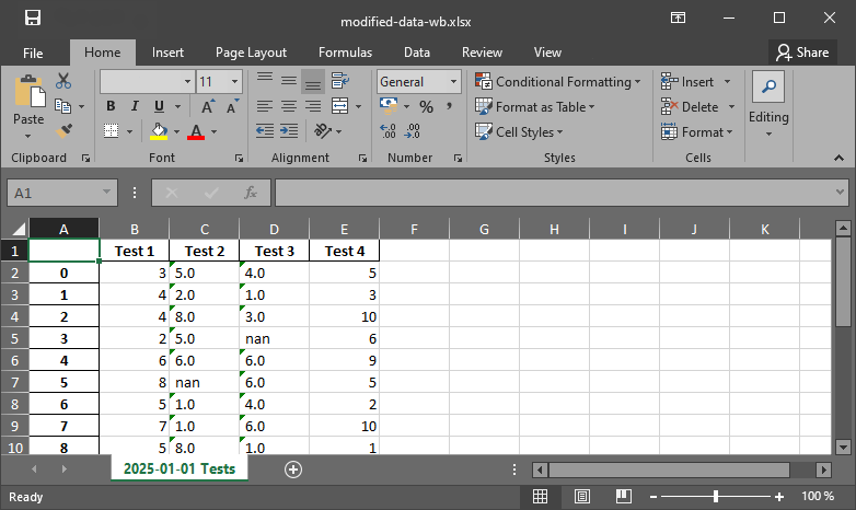
Figure 1:Die xlsx-ausgabedatei, die mit pandas produziert wurde.
Ein pandas ExcelWriter-Objekt kann erstellt werden, um mehrere pd.DataFrame-Objekte in eine Arbeitsmappe auf einem oder mehreren Blättern zu schreiben. Hier ist ein Beispiel, bei dem die nicht-numerischen "nan"-Strings in measurement_data durch np.nan ersetzt werden, um einen rein numerischen Datenrahmen in zwei Schritten zu erhalten (# (1) und # (2)):
measurement_data = measurement_data.replace("nan", np.nan, regex=True)  # (1) replace "nan" with np.nan
measurement_data = measurement_data.apply(pd.to_numeric)  # (2) convert all data to numeric

# write workbook with pd ExcelWriter object
with pd.ExcelWriter("data/modified-data-wb-EW.xlsx") as writer:
    measurement_data.to_excel(writer, sheet_name="2025-01-01 Tests")
    df.to_excel(writer, sheet_name="pandas example")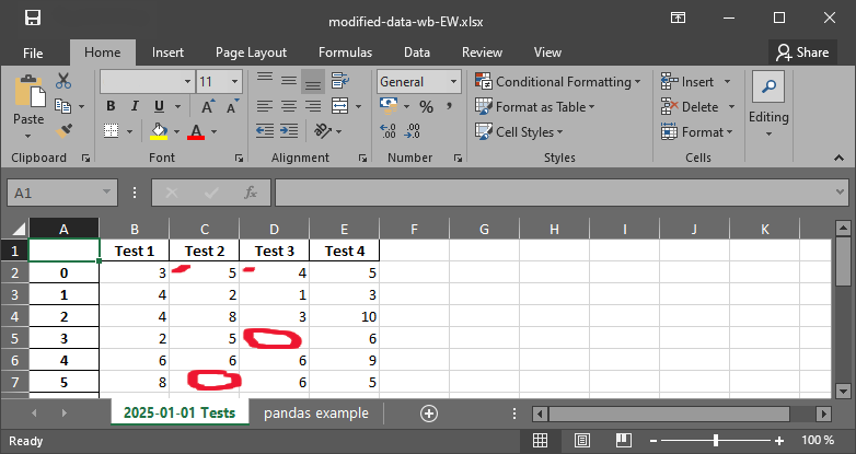
Figure 2:Die xlsx Datei mit Nan Strings.
Kategorisierte Daten
string-Variablen, die statistisch relevante Kategorien repräsentieren, sind die Basis für die Datenklassifizierung und -statistik. pandas stellt den speziellen Datentyp dtype="category" zur Verfügung, um statistische Analysen zu ermöglichen.
In the above Froude-number example, we used five categories to classify the flow regime as a function of the Froude number, which can serve as categories. This is useful, for instance, when no water was flowing or when a sensor broke in an experiment and we want to categorize our measurements to filter valid tests only:
flow_regimes = ["fluvial", "near-critical (slow)", "critical", "near-critical (fast)", "super-critical"]
observation_examples = ["fluvial", "dry", "critical", "near-critical (slow)", "measurement error"]
Fr_cat = pd.Categorical(observation_examples, categories=flow_regimes, ordered=False)
print(pd.Series(Fr_cat))
0 fluvial
1 NaN
2 critical
3 near-critical (slow)
4 NaN
dtype: category
Categories (5, str): ['fluvial', 'near-critical (slow)', 'critical', 'near-critical (fast)', 'super-critical']
/tmp/ipykernel_16649/2029032689.py:3: Pandas4Warning: Constructing a Categorical with a dtype and values containing non-null entries not in that dtype's categories is deprecated and will raise in a future version.
  Fr_cat = pd.Categorical(observation_examples, categories=flow_regimes, ordered=False)
Datenrahmenstatistik
pandas has efficient routines to perform workbook-like row or column sorting (e.g., df.sort_index() or df.sort_values()), and enables the fast calculation of data frame statistics with df.describe(), where 25%, 50%, and 75% represent the i-th percentiles:
measurement_data.describe()Statistische pandas Datenrahmenmethoden überschneiden sich mit NumPy Methoden und umfassen:
df.abs()berechnet absolute Wertedf.cumprod()calculates the cumulative productdf.cumsum()calculates the cumulative sumdf.count()counts the number of non-null observationsdf.max()calculates the maximum valuedf.mean()calculates the mean (average)df.min()berechnet den Mindestwertdf.mode()berechnet den Modusdf.prod()berechnet das Produktdf.std()berechnet die Standardabweichungdf.sum()berechnet die Summe
print("Mean:\n" + str(measurement_data.mean()))
print("Median:\n" + str(measurement_data.median()))
print("Standard deviation:\n" + str(measurement_data.std()))
Mean:
Test 1 2.785714
Test 2 3.266667
Test 3 2.900000
Test 4 3.062500
dtype: float64
Median:
Test 1 2.5
Test 2 3.0
Test 3 3.0
Test 4 3.0
dtype: float64
Standard deviation:
Test 1 1.423893
Test 2 1.032796
Test 3 1.197219
Test 4 1.611159
dtype: float64
Benutzerdefinierte (eigene) Funktionen auf Datenrahmen anwenden
pandas-Datenrahmen haben eine eingebaute apply(fun)-Methode, die es ermöglicht, eine benutzerdefinierte Funktion auf (Teile) eines pd.DataFrame-Objekts anzuwenden. Der folgende Codeblock leiht sich die Funktion feet_to_meter aus dem Kapitel functions aus (Download
from fun.converter import feet_to_meter

# create data frame with random integers
df = pd.DataFrame({"Feet": np.random.randint(0, 100, size=6),
                   "Meters": np.ones(6) * np.nan})

# apply feet_to_meter to the Meters columns of the data frame
df["Meters"] = df["Feet"].apply(feet_to_meter)

print(df)
Feet Meters
0 18 5.4864
1 62 18.8976
2 53 16.1544
3 95 28.9560
4 61 18.5928
5 59 17.9832
Termine und Uhrzeit
pandas involves methods for calculations and labeling with date and time values through pd.Timestamp, which converts date-time-like strings into timestamps or creates timestamps from keyword arguments:
print(pd.Timestamp('2025-01-01T12'))
print(pd.Timestamp(year=2025, month=1, day=1, hour=12))
print(pd.Timestamp(2025, 1, 1, 12))
2025-01-01 12:00:00
2025-01-01 12:00:00
2025-01-01 12:00:00
Der Ausdruck pd.Timestamp(2025, 1, 1, 12) ahmt das leistungsstarke datetime.datetime API (Application Programming Interface) der datetime Python-Bibliothek nach, die ausgeklügelte Methoden zum Umgang mit zeitabhängigen Werten bietet. Während pandas’ eingebaute Zeitstempel zum Erstellen von Zeitreihen in pd.DataFrame-Objekten und arbeitsmappenartigen Tabellen geeignet sind, ist datetime eine der besten Lösungen für zeitabhängige Berechnungen in Python. datetime ist standardmäßig verfügbar (d.h. es darf nicht conda oder pip-installiert sein) und ist effizient anwendbar, zum Beispiel auf Daten, die über mehrere Jahre einschließlich Schaltjahre gesammelt wurden. Das datetime Paket enthält viele Attribute und Methoden, die im Python docs] detailliert dokumentiert sind.
Die Standardverwendung ist:
import datetime as dt
start_date = dt.datetime(2024, 2, 25, 22, 30, 0)
end_date = dt.datetime(year=2024, month=3, day=2, hour=2, minute=15, second=30)
print("Datetime variables can be subtracted:\n" + str(end_date - start_date))
print("The result is a %s object." % type(end_date - start_date))
Datetime variables can be subtracted:
5 days, 3:45:30
The result is a <class 'datetime.timedelta'> object.
dt.timedelta Objekte können auch separat definiert werden:
time_diff = dt.timedelta(days=0, seconds=0, microseconds=0, milliseconds=0, minutes=0, hours=23, weeks=0)
act_time = start_date
print("Iterate from start to end date with stepsize=time_diff:")
while act_time <= end_date:
    print(act_time.strftime("%Y-%m(%h)-%d, %H:%M:%S"))
    act_time += time_diff
Iterate from start to end date with stepsize=time_diff:
2024-02(Feb)-25, 22:30:00
2024-02(Feb)-26, 21:30:00
2024-02(Feb)-27, 20:30:00
2024-02(Feb)-28, 19:30:00
2024-02(Feb)-29, 18:30:00
2024-03(Mar)-01, 17:30:00
Das ist alles für die Einführung in die Daten- und Dateiverarbeitung. Obwohl es viel mehr zur Datenverarbeitung gibt, als in diesem Kapitel gezeigt wird, und die nächsten anderen Kapitel dieses eBooks werden gelegentlich mehr Werkzeuge enthalten.