Run this notebook in your web browser: 
Der Link öffnet b10-xml.py als interaktives marimo Notebook, das vollständig in Ihrem Webbrowser läuft, ohne etwas zu installieren.
Warten Sie einen Moment, bis Python im Browser geladen ist (das dauert nur am ersten Start länger).
Klicken Sie auf die gelbe Starttaste (▶, unten rechts) um alle Zellen auszuführen.
Bearbeiten und re-run jede Codezelle zu experimentieren: marimo automatisch aktualisiert alle Zellen, die davon abhängig sind.
Ihre Bearbeitungen bleiben nur im Browser-Tab. Um sie zu halten, speichern Sie das Notizbuch durch das Menü (≠, oben rechts) > Export... > Python.
Run this marimo notebook locally
Um b10-xml.py auf Ihrem eigenen Gerät zu betreiben, erhalten Sie es vom marimo
Repository:
git clone https://github.com/sschwindt/marimo-python-course.gitDie Kursumgebung erstellen und aktivieren:
conda env create -f environment.ymlundconda activate hy-marimoStarten Sie im Ordner Repository das Notebook mit
marimo edit b10-xml.py
Run this notebook with Jupyter
This page is also available as the Jupyter notebook b10-xml.ipynb in the jupyter , or install Python and JupyterLab locally to run b10-xml.ipynb on your own machine.
Erstellen, Manipulieren und Kopieren von semistrukturierten Datendateien in Form von xlsx-Workbooks und JSON-Dateien: Dieses Kapitel beginnt mit Hintergrundinformationen über XML und was XML mit Arbeitsmappen zu tun hat, und JSON: XML ist eine Abkürzung für Ex tensible Markup Language, die Regeln für die Kodierung von Dokumenten definiert]. XML ist eine textbasierte Auszeichnungssprache zur Darstellung von Dokumentenstruktur und Daten. Eine XLSX-Arbeitsmappe ist ein Office Open XML-Paket: Sie wird normalerweise als ZIP-Archiv mit XML-Teilen und anderen Ressourcen gespeichert. Anwendungen wie Tabellenkalkulationsprogramme interpretieren diese Teile und präsentieren den Benutzern die Arbeitsmappe. HTML hat seine eigene Syntax und Parsing-Regeln, obwohl HTML auch mit XML-Syntax serialisiert werden kann. Andere strukturierte Dateiformate wie JSON (JavaScript Object Notation) ist ein separates Textformat, das strukturierte Daten mit Objekten, Arrays, Strings, Zahlen, booleschen Werten und Null darstellen kann.
Der Umgang mit strukturierten Daten ist wichtig in der Wasserressourcentechnik, wo wir in der Praxis oft am Austausch von Informationen mit Managern interessiert sind, die Büroarbeitsmappen (.xlsx Dateien) bevorzugen. Außerdem können JSON-Dateien numerische Modelle effizient speichern (z. B. für BASEMENT).
Watch this section as a video
Watch this section as a video on the @Hydro-Morphodynamics channel on YouTube.
Arbeitsbuch (xlsx)
Warum wollen wir überhaupt mit Arbeitsmappen kommunizieren? Wir haben bereits gesehen, dass Python viel leistungsfähiger ist als Office-Programme zur systematischen Analyse von Daten. Python erfordert jedoch die Abstraktion von Daten in unseren Köpfen, um beispielsweise die Struktur einer verschachtelten Liste zu visualisieren. Aus diesem Grund müssen Daten von und für das Marketing, Ihren Chef oder Behörden oft optisch einfach zu bedienende Arbeitsmappenformate haben, die schnell übersehen werden können. Dennoch wollen wir den Inhalt solcher Arbeitsmappeninformationen effizient mit Python nutzen und wir wollen visuell einfache Ausgaben erzeugen, die jeder ohne Python-Kenntnisse lesen kann.
Wir haben bereits gesehen, dass pandas einfache Routinen zum Importieren und Exportieren von Daten aus bzw. in Arbeitsmappen bietet (vgl. file reading and writing with pandas). pandas verwendet in erster Linie openpyxl, je nachdem, was in der aktiven Python-Umgebung verfügbar ist]. openpyxl ist eine der mächtigsten Optionen für den Umgang mit Arbeitsmappen mit Python (Anmerkung: diese Behauptung ist subjektiv) und dieser Abschnitt führt openpyxl ein.
Diese Einleitung verwendet die folgenden arbeitsmappenbezogenen Begriffe:
workbook ist die Hauptxlsx-Datei, mit der wir arbeiten (auch spreadsheet genannt);
sheet ist der tabellarische Inhalt einer Arbeitsmappe und eine Arbeitsmappe kann mehrere Blätter haben;
** Spalte**s sind vertikale Linien in einem Blatt;
rows sind horizontale Linien in einem Blatt;
cells sind Elemente eines Blattes.
Ein Arbeitsbuch erstellen
openpyxl has a Workbook class that enables to create and fill workbooks with data. Typically, an instance of the Workbook class is called wb, and worksheet variables are called ws.
import numpy as np
import openpyxl as oxl


wb = oxl.Workbook()  # create a Workbook instance
ws = wb.active  # activate worksheet
ws.title = "Gaussian 2D"  # name worksheet
ws["A1"] = "Gaussian sample data"  # write to cell A1

# generate some data
x, y = np.meshgrid(np.linspace(-1, 1, 20), np.linspace(-1, 1, 20))
dis = np.sqrt(x * x + y * y)
sigma, mu = 1.0, 0.0
gaussian = np.exp(-((dis - mu) ** 2 / (2.0 * sigma ** 2)))

# write data to worksheet
m, n = gaussian.shape
for i in range(1, m + 1):
  for j in range(1, n + 1):
	  ws.cell(row=i + 1, column=j, value=gaussian[i - 1, j - 1])

print("Workbook data in cell A2: "+ str(ws["A2"].value))
print("Corresponds to np.array value: " + str(gaussian[0, 0]))

# save and close (destruct object) workbook
wb.save(filename="data/python_workbook.xlsx")
wb.close()
Workbook data in cell A2: 0.3678794411714422
Corresponds to np.array value: 0.3678794411714422
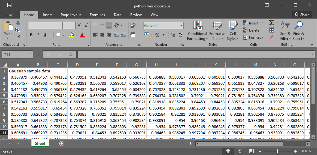
Figure 1:Das resultierende Arbeitsbuch.
Lesen und manipulieren eines vorhandenen Arbeitsbuchs
openpyxl.load_workbook(...) akzeptiert Optionen wie:
read_only=Truefür eine speichereffiziente, schreibgeschützte Ansicht einer vorhandenen Arbeitsmappe;data_only=Falseto expose formula text, ordata_only=Trueto expose the cached value last stored by a spreadsheet application;keep_vba=Trueto preserve VBA content without making it editable.
Schreibmodus gilt beim Erstellen einer neuen Arbeitsmappe: openpyxl.Workbook(write_only=True).
If read_only=False, we can manipulate cell values and also cell formats, including data formats (e.g., date, time, and many more), font properties (and many more cell styles), or colors in HEX Color Code (find your favorite color here). The following example opens the above-created python_workbook.xlsx, adds a new worksheet, illustrates the implementation of cell styles, and fills the workbook with random discharge measurements.
import datetime
from openpyxl.styles import Font, Alignment, PatternFill
wb = oxl.load_workbook(filename="data/python_workbook.xlsx", read_only=False)
ws = wb.create_sheet(title="Discharge")

# define title styles
title_font = Font(name="Tahoma", size="11", bold=True, italic=True, color="C1D0DE")
title_fill = PatternFill(fill_type="solid", start_color="050505", end_color="073AD4")
title_align = Alignment(horizontal='center', vertical='bottom', text_rotation=0,
                        wrap_text=False, shrink_to_fit=False, indent=0)

date_time_format = "yyyy-mm-dd hh:mm:ss"
ws["A1"] = "Date-Time (%s)" % date_time_format

title_cell_flow = ws["B1"]
title_cell_flow.value = "Discharge (CMS)"
title_cell_flow.font = title_font
title_cell_flow.fill = title_fill
title_cell_flow.alignment = title_align

# define time period and time delta of 1 hour = 3600 seconds
current_date_time = datetime.datetime(2040, 12, 24, 0, 0)
dt = datetime.timedelta(seconds=3600)

# write random discharges to workbooks
for row in ws.iter_rows(min_row=2, max_row=26, min_col=1, max_col=2):
    row[0].value = current_date_time
    row[0].number_format = date_time_format
    row[1].value = np.random.random_sample(size=None) * 100
    row[1].number_format = "0.00"
    current_date_time += dt

wb.save("data/python_workbook_reloaded.xlsx")
wb.close()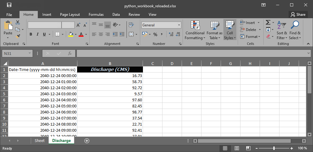
Figure 2:Die aktualisierte Arbeitsmappe.
The below code block provides the short helper function read_columns to read only one or more columns into a (nested) list (reads until the maximum number of rows, defined by ws.rows, in a workbook is reached). A similar function can be written for reading rows.
def read_columns(ws, start_row=1, columns="ABC"):
  """Return one list per requested worksheet column."""
  return [
	  [ws[f"{column}{row}"].value
	   for row in range(start_row, ws.max_row + 1)]
	  for column in columns
  ]


# example usage:
wb = oxl.load_workbook(filename="data/python_workbook.xlsx", read_only=False)
ws = wb.active
col_D = read_columns(ws, start_row=2, columns="D")
col_F = read_columns(ws, start_row=2, columns="F")
wb.close()
Challenge: Add a random test set to modified-data-wb.xlsx
The pandas file handling section features the creation of a workbook containing 4 columns of test data (download modified-data-wb.xlsx). For a random-test comparison, you want to add a column of random values. To this end:
Öffnen Sie modified-data-wb.xlsx mit openpyxl
wb = oxl.load_workbook(filename="data/modified-data-wb.xlsx", read_only=False)Holen Sie sich das aktive Arbeitsblatt
ws = wb.activeFügen Sie einen neuen Spaltennamen in Spalte F hinzu:
ws["F1"].value = "Random values"Erstellen Sie eine Liste (dh ein 1d-Array) von Zufallszahlen mit numpy (vergessen Sie nicht
import numpy as np)rnd_data = np.random.random(18)Iterieren Sie über das zufällige Datenfeld und schreiben Sie die Werte in die Spalte F der Arbeitsmappe
Start the iteration with
for row, val in enumerate(rnd_data):In every iteration add the next random value of
rnd_datawithws["F" + str(row + 2)].value = val
Note the usage ofrow + 2(one header column and different absolutes of Python and the workbook)
Speichern und Schließen der Arbeitsmappe
wb.save(os.getcwd() + "/data/re-modified-data-wb.xlsx"(vergiss nichtimport os)wb.close()Verwenden Sie alternativ einen Namensraum für die Manipulation der Arbeitsmappe!
Formeln in Arbeitsmappe
openpyxl can read and write formula strings, but it does not calculate them. With data_only=False, a formula cell exposes its formula text. With data_only=True, it exposes the cached result last stored by a spreadsheet application, which may be missing or stale. Membership in openpyxl.utils.FORMULAE can be informative, but it does not evaluate or validate a formula. However, not all workbook formulae are recognized by openpyxl and in the case of doubts, a dirty try-and-error approach is the only remedy. As an example, change SQRT in the below example to the formula in question. However, not all workbook formulae are recognized by openpyxl and in the case of doubts, a dirty try-and-error approach is the only remedy. As an example, change SQRT in the below example to the formula in question.
from openpyxl.utils import FORMULAE
print("SQRT" in FORMULAE)
True
(Un)
Das Zusammenführen und Entschmelzen von Zellen ist eine beliebte Bürofunktion für Stilzwecke und openpyxl bietet auch Funktionen zum Durchführen von Fusionsoperationen:
ws.merge_cells(start_row=1, end_row=3, start_column=1, end_column=2)
ws.unmerge_cells(start_row=1, end_row=3, start_column=1, end_column=2)
Diagramme (Plotten)
In the unlikely event that you want to insert plots directly into workbooks with Python (matplotlib is more powerful anyway), openpyxl provides features for this purpose as well. To illustrate the creation of an area chart, the below code block re-uses the first column of random values in the above-created python_workbook.xlsx.
from openpyxl.chart import AreaChart, Reference, Series

wb = oxl.load_workbook(filename="data/python_workbook.xlsx", read_only=False)
ws = wb.active

chart = AreaChart()
chart.title = "Random Gaussian"
chart.style = 10
chart.x_axis.title = "Cell row"
chart.y_axis.title = "Random value (-)"

col_D = Reference(ws, min_col=4, min_row=2, max_row=20)
col_F = Reference(ws, min_col=6, min_row=2, max_row=20)

chart.add_data(col_F, titles_from_data=False)
chart.add_data(col_D, titles_from_data=False)

ws.add_chart(chart, "B2")

wb.save("data/python_workbook_chart.xlsx")
wb.close()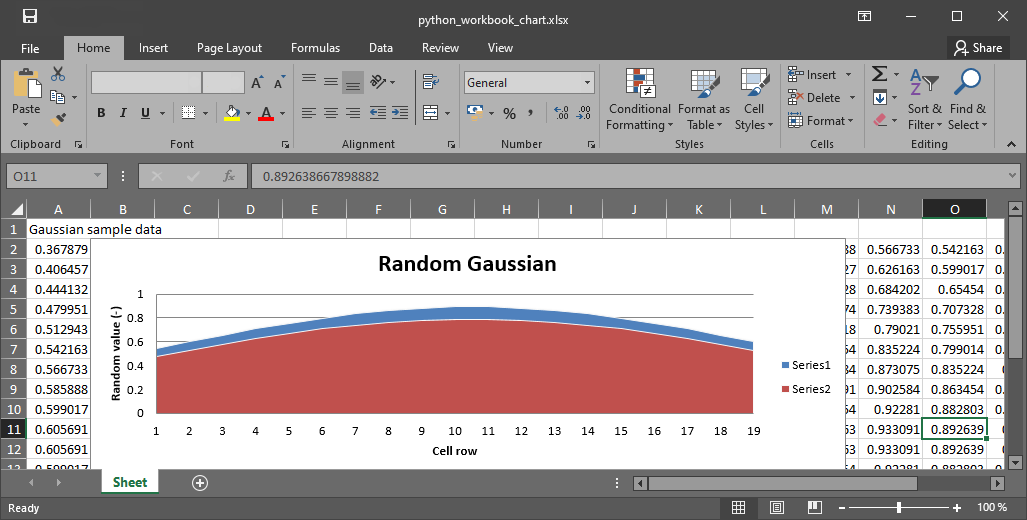
Figure 3:Die Arbeitsmappe mit dem in Python erstellten Plot.
Andere Arbeitsmappendiagramme sind verfügbar und ihre Implementierung (immer noch: Warum sollten Sie?) wird im openpyxl docs] erklärt.
Workbook Manipulation anpassen
There are many ways of modifying workbooks and openpyxl provides close-to “shovel-ready” methods to manipulate a workbook. Still, to avoid re-reading this lesson every time you want to manipulate a workbook, it is more convenient to have your own workbook manipulation classes ready to work. To this end, the following code block defines custom Read and Write classes, where Read is the parent class of the Write class (recall the section on inheritance of classes). The Read class may contain tailored functions for reading specific columns, rows, or arrays. The below code block also makes use of the above-defined read_columns function, implemented as a method of the Read class.
import openpyxl as oxl


class Read:
  def __init__(self, workbook_name, *, read_only=False,
			   data_only=False, sheet_name=None):
	  self.wb = oxl.load_workbook(
		  filename=workbook_name,
		  read_only=read_only,
		  data_only=data_only,
	  )
	  self.ws = self.wb[sheet_name] if sheet_name else self.wb.active

  def read_columns(self, start_row=1, columns="ABC"):
	  return [
		  self.ws[f"{column}{row}"].value
		  for row in range(start_row, self.ws.max_row + 1)
		  for column in columns
	  ]


  def __call__(self):
	  print(dir(self))


class Write(Read):
  def __init__(self, workbook_name, *, data_only=False,
			   sheet_name=None):
	  super().__init__(
		  workbook_name,
		  read_only=False,
		  data_only=data_only,
		  sheet_name=sheet_name,
	  )
An extended example script with more complex Read and Write classes can be downloaded from the course repository.
Ein Beispiel aus der Wasserressourcentechnik und Forschung
The ecological restoration or enhancement of rivers requires, among other data, information on preferred water depths and flow velocities of target fish species. This information is established by biologists and then often provided in the shape of so-called habitat suitability index (HSI) curves in workbook formats. Typically, we produce geospatially explicit data on water depth and flow velocity with numerical models. The output of two or three-dimensional numerical models is way too large to be handled with office applications. So we need an advanced tool, such as Python, to handle the geospatially explicit data, and read and interpolate HSI curves from workbooks. What does that look like technically? The exercises on geospatial Python will let you dive into aquatic habitat (assessments).
JSON
JavaScript Object Notation (JSON) files have a similar structure to XML and enable the structured storage of (human-readable) data. For instance, the numerical code BASEMENT v.3.x (read more in the numerical modeling chapter) uses a model.json and a simulation.json file to store model setup parameters such as material properties. Thus, automating numerical model setups with Python involves the modification of model parameters stored in json files. This is where Python steps in with the standard-library json module that encodes and decodes JSON. JSON values can be objects, arrays, strings, numbers, true, false, or null. An object contains string names paired with values, for example {"name": "Vanilla Flow"}. An array is an ordered sequence of values, for example [1, 3, 7, 31].
JSON-Dateistruktur
A JSON file consists of two types of data structures, which are dictionary objects and arrays in the form of lists of values. The dictionary objects in a JSON file correspond to the same format that we already know in Python: Pairs of keys (names) and values embraced by curly brackets (braces) {"name": value}. The value can be a string, numeric, a comma-separated list [] (array) of data, or another dictionary.
The following example shows a JSON file called river_struct.json with a RIVER key that has a nested dictionary as a value. The value-dictionary contains three keys (NAME, GEOMETRY, and HYDRAULICS).
{
	"RIVER": {
		"NAME": "Vanilla Flow",
		"GEOMETRY": {
			"REGIONS": [
				{
				  "type": "wet",
				  "name": "riverbed"
				},
				{
				  "type": "dry",
				  "name": "floodplain"
				}
			],
			"FLOWBOUNDARIES": [
				{
				  "name": "Inflow",
				  "nodes": [1, 3, 7, 31]
				},
				{
				  "name": "Outflow",
				  "nodes": [89, 90, 76, 69, 95]
				}
			]
		},
		"HYDRAULICS": {
			"BOUNDARY": [
				{
					"discharge_file": "/simulation/directory/Inflow.txt",
					"name": "Inflow",
					"slope": 0.005,
					"type": "hydrograph"
				},
				{
					"name": "Outflow",
					"type": "zero_gradient"
				}
			],
			"FRICTION": {
				"cobble": 20.0,
				"gravel": 26.0,
				"sand": 41
			}
		},
		"LOCATION": [48.744079, 9.103928]
	}
}
{'RIVER': {'NAME': 'Vanilla Flow',
'GEOMETRY': {'REGIONS': [{'type': 'wet', 'name': 'riverbed'},
{'type': 'dry', 'name': 'floodplain'}],
'FLOWBOUNDARIES': [{'name': 'Inflow', 'nodes': [1, 3, 7, 31]},
{'name': 'Outflow', 'nodes': [89, 90, 76, 69, 95]}]},
'HYDRAULICS': {'BOUNDARY': [{'discharge_file': '/simulation/directory/Inflow.txt',
'name': 'Inflow',
'slope': 0.005,
'type': 'hydrograph'},
{'name': 'Outflow', 'type': 'zero_gradient'}],
'FRICTION': {'cobble': 20.0, 'gravel': 26.0, 'sand': 41}},
'LOCATION': [48.744079, 9.103928]}}Lesen (decode) und schreiben (encode) JSON-Dateien mit der json Bibliothek
JSON files can be implemented in many programming languages, including HTML and Python. Python has a built-in json library that enables JSON decoding and encoding. The json library provides a json.dumps(DATA) method to “dump” (i.e., encode) data in JSON format. Vice versa, the json.load() function reads data from JSON files.
The following example illustrates encoding and decoding an arbitrarily nested dataset with the json library.
import json
# create arbitrary nested data (list, dictionary, tuple)
data_for_json = [
  "list_element1",
  {"dict_key": ("tuple_element", "text", 1.0, None)},
]

# create a json file
json_file = open("data/my-first.json", mode="w+")
# encode the random nested data list in json format and write to file
json_file.write(json.dumps(data_for_json))
# close file
json_file.close()

# re-open the json file to read data
with open("data/my-first.json", mode="r") as re_opened_file:
    raw_data = re_opened_file.readline()

# decode json data in a Python variable
data_from_json = json.loads(raw_data)
print(json.dumps(data_from_json))
["list_element1", {"dict_key": ["tuple_element", "text", 1.0, null]}]
Die Python docs] bietet weitere Optionen und Beschreibungen zur Verwendung der json-Bibliothek. Hier werden wir jedoch (wieder einmal) die pandas-Bibliothek nutzen, die leistungsstarke Funktionen für den Umgang mit Json-Daten bietet.
Lesen (decode) und schreiben (encode) JSON-Dateien mit pandas
pandas (recall data and file handling with pandas) ermöglicht das Lesen von JSON-Dateien in das bequeme Tabellenformat mit einer eingebetteten Verwendung der json-Bibliothek. Der folgende Codeblock verwendet die Funktion pandas.read json(FILE)], um die oben gezeigte RIVER Beispieldatei zu lesen (download river struct.json).
import pandas as pd
river = pd.read_json("data/river_struct.json")
print(river)
RIVER
NAME Vanilla Flow
GEOMETRY {'REGIONS': [{'type': 'wet', 'name': 'riverbed...
HYDRAULICS {'BOUNDARY': [{'discharge_file': '/simulation/...
LOCATION [48.744079, 9.103928]
Since a river without data is like ice cream without taste, we will add (random) data on flow characteristics to the data structure. Let’s assume that we have used the data from river_struct.json to simulate a stationary discharge in a two-dimensional numerical model. As a result, we have two regular grids (arrays) with data on flow velocity and water depth. Now, we want to append both the flow velocity and water depth arrays in the form of a result structure (dictionary) to river_struct.json and give the river a new name.
# create random data
import numpy as np
h = np.random.weibull(np.arange(0,100)).reshape(10, 10)
u = np.random.weibull(np.arange(0,100)).reshape(10, 10)

# append RESULTS row to pandas dataframe
river_dict = river.to_dict()
river_dict["RIVER"].update({"RESULTS": {"water_depth": h, "flow_velocity": u}})
updated_river = pd.DataFrame.from_dict(river_dict)

# re-NAME RIVER
updated_river.loc["NAME", "RIVER"] = "Honey river"
print(updated_river)

# export to JSON
updated_river.to_json("data/river_results.json")
RIVER
NAME Honey river
GEOMETRY {'REGIONS': [{'type': 'wet', 'name': 'riverbed...
HYDRAULICS {'BOUNDARY': [{'discharge_file': '/simulation/...
LOCATION [48.744079, 9.103928]
RESULTS {'water_depth': [[0.0, 1.4016850027236283, 0.6...
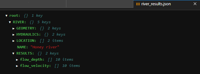
Figure 4:Das resultierende Arbeitsbuch.