Machen Sie sich bereit, indem Sie das Übungsrepository klonen:
git clone https://github.com/Ecohydraulics/Exercise-SedimentTransport.git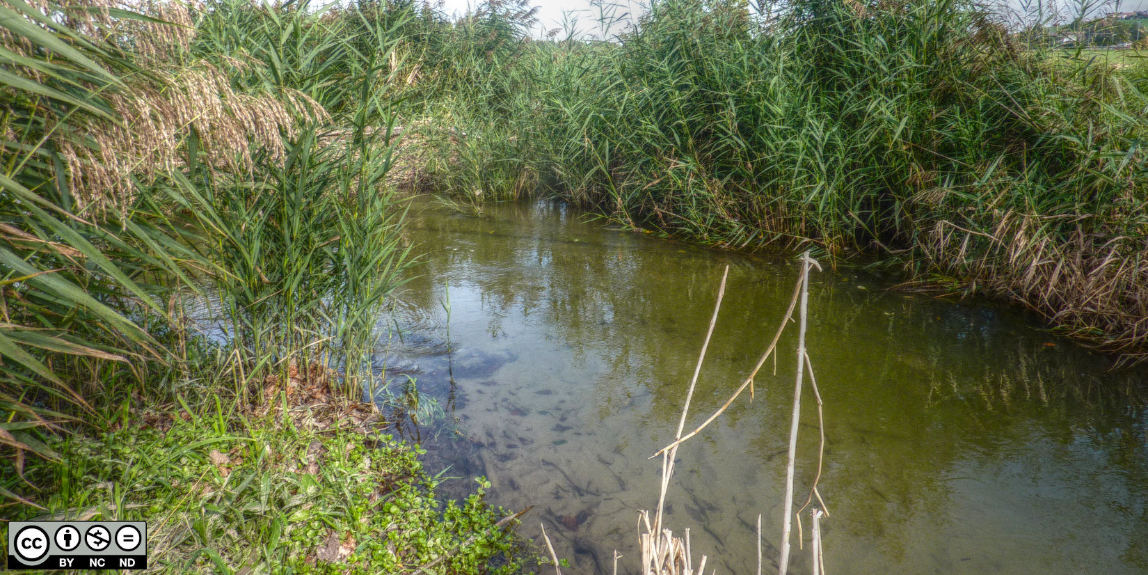
Figure 1:Die Arbogne in der Schweiz (Quelle: Sebastian Schwindt 2013).
Theorie
1d Querschnitt gemittelte Hydrodynamik
Anhand der Stufenentladung (Manning-Strickler Formel) exercise erinnern wir uns an die Formel, um die Beziehung zwischen der Wassertiefe (inklusive des hydraulischen Radius ) und der Strömungsgeschwindigkeit zu berechnen:
wo
ist die Manning coefficient in fiktionalen Einheiten von (s/m).
ist die hypothetische Energieschrägheit (m/m) und entspricht der Kanalschrägheit für stetige, gleichmäßige Strömungsverhältnisse (in natürlichen Flüssen nicht vorhanden).
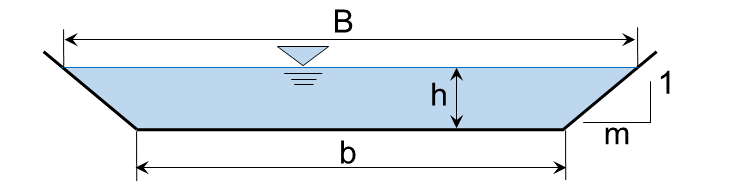
hydraulic radius , where (for a trapezoidal cross-section):
the wetted (trapezoidal) cross-section area is ;
the wetted perimeter of a trapezoid is ;
(channel base width) and (bank slope) are illustrated in the figure below to calculate the depth-dependent water surface width .
This exercise uses one-dimensional (1d) cross-section averaged hydraulic data produced with the US Army Corps of Engineers HEC-RAS software U.S. Army Corps of Engineeers, 2016, which solves the Manning-Strickler formula numerically for any flow cross-section shape. In this exercise, HEC-RAS provides the hydraulic data needed to determine the Sedimenttransport capacity of a channel cross-section, although no explanations for creating, running, and exporting data from HEC-RAS models are given.
Sedimenttransport
Fluvial Sedimenttransport can be distinguished into two modes: (1) Schwebstoff and (2) Geschiebe (see Fig. 3). Finer particles with a weight that can be carried by the fluid (water) are transported as Schwebstoff. Coarser particles rolling, sliding, and jumping on the channel bed are transported as Geschiebe. There is another type of transport, the so-called wash load, which is finer than the coarse Geschiebe, but too heavy (large) to be transported in suspension Einstein, 1950.
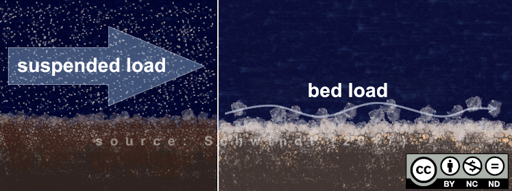
Figure 3:Zwei Arten des Sedimenttransports (Quelle: Schwindt, 2017).
In the following, we will look at the Geschiebe transport mode. In this case, a sediment particle located in or on the riverbed is mobilized by shear forces of the water as soon as they exceed a critical value (see figure below). In river hydraulics, the so-called dimensionless bed shear stress or Shields stress Shields, 1936 is often used as the threshold value for the mobilization of sediment from the riverbed (see Fig. 4). This exercise uses one of the dimensionless bed shear stress approaches and the next section provides more explanations.
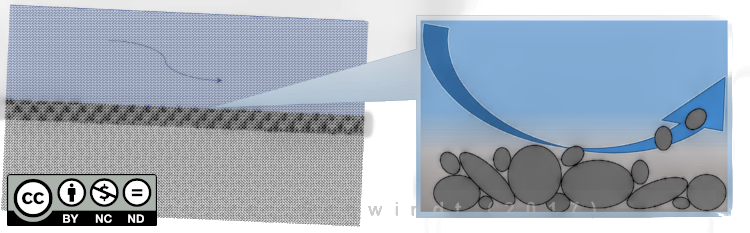
Figure 4:Das Prinzip der Sedimentmobilisierung.
Die Meyer-Peter und Müller (1948) Formel
The Meyer-Peter & Müller (1948) formula for estimating Geschiebe transport was published by Swiss researchers Eugen Meyer-Peter (founder of the Laboratory of Hydraulics, Hydrology and Glaciology (VAW) and Robert Müller. Their study began one year after the establishment of the VAW in 1931 when Robert Müller was appointed assistant to Eugen Meyer-Peter. The two scientists worked in collaboration with Henry Favre and Albert Einstein’s son Hans Albert. In 1934, the laboratory published for the first time a formula for the calculation of Geschiebe transport and its fundamental relationship between observed and critical dimensionless bed shear stresses is used until today. The dimensionless Geschiebe transport rate according to Meyer-Peter & Müller (1948) is:
Die übrigen Parameter sind:
2.68, the dimensionless ratio of sediment grain density ( 2680 kg/m³) and water density ( 1000 kg/m³);
, the characteristic grain size in (m). It can be assumed that (i.e., the grain diameter of which 84% of a sediment mixture is smaller) in line with the scientific literature (e.g., Rickenmann & Recking (2011)).
The Meyer-Peter & Müller formula applies (like any other Sedimenttransport formula) only to certain rivers that have the following characteristics (range of validity):
0.4 10 m < 28.6 10 m
10 m 639 ( denotes the dimensionless Froude-Zahl)
0,0004 0,02
0,0002 m/(s m) 2.0 m/(s m) ( ist die Entladung der Einheit, d.h. )
0.25 3.2
The dimensionless expression for Geschiebe was used to enable information transfer between different channels across scales by preserving geometric, kinematic, and dynamic similarity. The set of dimensionless parameters used results from Buckingham’s theorem Buckingham, 1915. Therefore, to add dimensions to , it needs to be multiplied with the same set of parameters used for deriving the dimensionless expression from Meyer-Peter & Müller. Their set of parameters involves the characteristic grain size , the grain density , and the gravitational acceleration . Thus, the dimensional unit Geschiebe is (in kg/s and meter width, i.e., kg/(sm):
The cross-section averaged Geschiebe (kg/s) is then:
wobei die hydraulisch aktive Kanalbreite des Strömungsquerschnitts ist (z. B. für ein Trapez ).
Code
Legen Sie den Rahmen
Der objektorientierte Code verwendet benutzerdefinierte Klassen, die wir in einem main.py Skript aufrufen. Erstellen Sie die folgenden zusätzlichen Skripte, die die benutzerdefinierten Klassen und Funktionen zur Steuerung der Protokollierung enthalten.
fun.pyenthält Protokollierungsfunktionen.hec.pywird eineHecSetKlasse enthalten, um hydraulische Ausgabedaten von HEC-RAS als strukturierte Objekte zu lesen.grains.pywird eineGrainReaderKlasse enthalten, um Informationen zur Korngrößenklasse als strukturierte Objekte zu lesen.bedload.pyenthält die KlasseBedCoremit grundlegenden Elementen, die die meisten Geschiebe Formeln gemeinsam haben.mpm.pyenthält die KlasseMPM, die vonBedCoreerbt und Geschiebe wie oben beschrieben berechnet (Meyer-Peter & Müller 1948).
Wir erstellen die Klassen und Funktionen in den angegebenen Skripten gemäß dem folgenden Flussdiagramm:
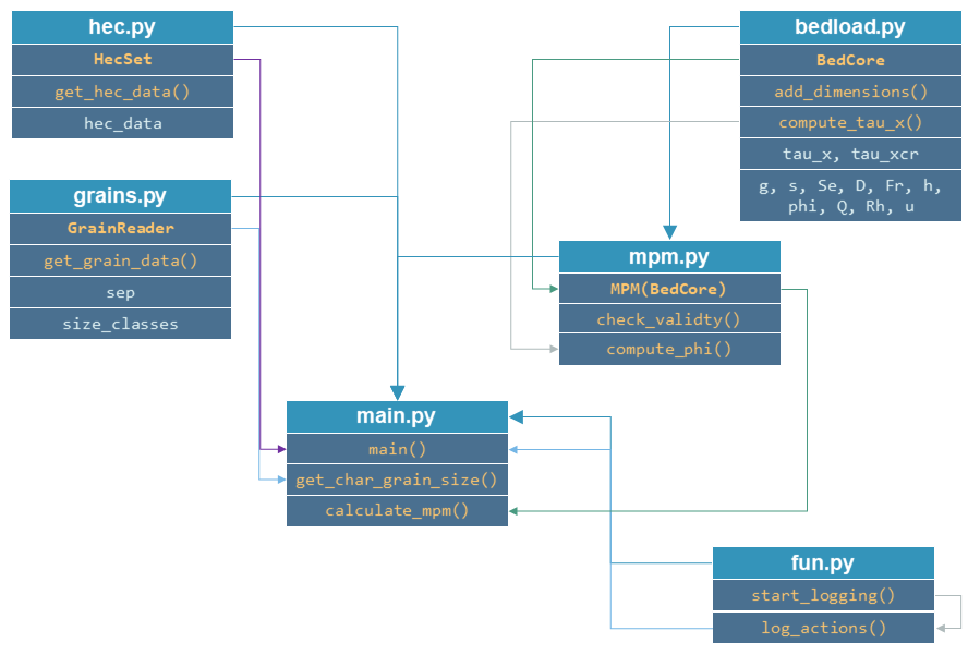
To start with the main.py script, add a main function as well as a get_char_grain_size and a calculate_mpm function. Moreover, make the script stand-alone executable:
# This is main.py
import os


def get_char_grain_size(file_name, D_char):
    return None


def calculate_mpm(hec_df, D_char):
    return None


def main():
    pass


if __name__ == '__main__':
    main()
Protokollierungsfunktionen
Das fun.pyScript enthält zwei Funktionen:
start_loggingzum Einrichten von Protokollierungsformaten und eines Logdateinamens, wie im Abschnitt unter logging beschrieben, undlog_actions, das ist ein Funktions-Wrapper für diemain()(main.py) Funktionen zum Protokollieren von Skriptausführungsnachrichten.
Die Funktion start_logging sollte so aussehen (ändern Sie den Namen der Logdatei, falls gewünscht):
import logging


def start_logging():
    logging.basicConfig(filename="logfile.log", format="[%(asctime)s] %(message)s",
                        filemode="w", level=logging.DEBUG)
    logging.getLogger().addHandler(logging.StreamHandler()
Die Wrapper-Funktion log_actions folgt den Anweisungen von functions theory section:
def log_actions(fun):
    def wrapper(*args, **kwargs):
        start_logging()
        fun(*args, **kwargs)
        logging.shutdown()
    return wrapper
To use the log_actions wrapper throughout the program, we will implement it at the highest level, which is the main() function in main.py:
# main.py
from fun import *

...

@log_actions
def main():
    logging.info("This is a test message (do not keep in the function).")


if __name__ == '__main__':
    main()
Now, we can log messages at different levels (info, warning, error, or others) in all functions called within main() by using for example logging.info("Message"), logging.warning("Message"), or logging.error("Message") rather than the print() function.
Lesen Sie Korngrößendaten
Sediment grain size classes (ranging from to ) are provided in the file grains.csv (delimiter=",") and can be customized.
Write a GrainReader class that uses the read_csv method from Pandas to read the grain size distribution from grains.csv. Write the class in a separate Python script (e.g., grains.py as indicated in the above figure):
class GrainReader:
    def __init__(self, csv_file_name="grains.csv", delimiter=","):
        self.sep = delimiter
        self.size_classes = pd.DataFrame
        self.get_grain_data(csv_file_name)
The get_grain_data method should look like this for reading the provided grain size classes:
    def get_grain_data(self, csv_file_name):
        self.size_classes = pd.read_csv(csv_file_name,
                                        names=["classes", "size"],
                                        skiprows=[0],
                                        sep=self.sep,
index_col=["classes"])Implement the instantiation of a GrainReader object in the main.py script in the get_char_grain_size function. The function should receive the string-type arguments file_name (here: "grains.csv") and D_char (i.e., the characteristic grain size to use from grains.csv). The main() function calls the get_char_grain_size function with the arguments file_name=os.path.abspath("..") + "\\grains.csv" and D_char="D84" (corresponds to the first column in grains.csv).
# main.py
import os
from grains import GrainReader

def get_char_grain_size(file_name=str, D_char=str):
    grain_info = GrainReader(file_name)
    return grain_info.size_classes["size"][D_char]

...

@log_actions
def main():
    # get characteristic grain size = D84
    D_char = get_char_grain_size(file_name=os.path.abspath("..") + "\\grains.csv",
                                 D_char="D84")
HEC-RAS Eingabedaten lesen
The provided HEC-RAS dataset is stored in the xlsx workbook HEC-RAS/output.xlsx and contains the following output:
| Col.No. | Alphabetic Col. | Variable | Type/Unit |Beschreibung | |--------------------------------------------------------------------------------------------------------------------------------------------------------------------------------------------------------------------------------------------------------------- | Col. 01 | A | Reach | string | River (reach) name | | Col. 02 | B | River Sta | [m] | Position auf der Längsachse des Flusses | | Spalte 03 | C | Profile | string | Name of flow scenario profile (z. B. HQ2.33) | | Spalte 04 | D | Q Total | [m3/s] | Flussableitung | | Spalte 05 | E | Min Ch El | [m a.s.l.] | Mindesthöhe (Niveau) des Kanalquerschnitts | | Col. 06 | F | W.S. Elev | [m a.s.l.] | Wasseroberflächenhöhe (Ebene) | | Spalte 07 | G | Vel Chnl | [m] | Strömungsgeschwindigkeit Hauptkanal | | Spalte 08 | H | Flow Area | [m2] | Benetzte Querschnittsfläche A (siehe oben) | | Spalte 09 | I | Froude# Chl | [-] | Froude-Zahl des Kanals (wenn 1, Berechnungsfehler - nicht verwenden!) | | Spalte 10 | J | Hydraulikradius | [m] | Hydraulikradius | | Spalte 11 | K | Hydr Tiefe | [m] | Wassertiefe (aktiver Querschnittsmittelwert) | | Spalte 12 | L | E.G. Slope | [m/m] | Energy Gradeline Hang |
Um HEC-RAS-Ausgabedaten zu laden, schreiben Sie eine benutzerdefinierte Klasse (in einem separaten Skript namens hec.py), die den Dateinamen als Eingabeargument annimmt und die HEC-RAS-Datei als pandas-Datenrahmen liest:
class HecSet:
    def __init__(self, xlsx_file_name="output.xlsx"):
        self.hec_data = pd.DataFrame
        self.get_hec_data(xlsx_file_name)
The get_hec_data method should look (something) like this:
    def get_hec_data(self, xlsx_file_name):
        self.hec_data = pd.read_excel(xlsx_file_name,
                                      skiprows=[1],
                                      header=[0])
Um ein HecSet-Objekt in der Funktion main() (main.py) zu erstellen, müssen wir es importieren und instanziieren, beispielsweise als hec = HecSet(file_name). Darüber hinaus können wir bereits die Weitergabe der pd.DataFrame der HEC-RAS-Daten an die calculate_mpm-Funktion (auch in main.py) implementieren, die wir später abschließen werden.
# main.py
import os
from ...
from hec import HecSet

...

@log_actions
def main():
    D_char = ...

    hec_file = os.path.abspath("..") + "{0}HEC-RAS{0}output.xlsx".format(os.sep)
    hec = HecSet(hec_file)
Erstellen Sie eine Beladungskernklasse
A BedCore class written in the bedload.py script provides variables and methods, which are relevant to many Geschiebe and Sedimenttransport calculation formulae, such as the Parker-Wong correction Wong & Parker, 2006 or the Smart & Jaeggi (1983) (direct download ). Moreover, the BedCore class contains constants such as the gravitational acceleration (i.e., self.g=9.81), the ratio of sediment grain and water density (i.e., self.s=2.68), and the critical dimensionless bed shear stress (i.e., self.tau_xcr=0.047, which may be re-defined by users). The header of the BedCore class should look (similar) like this:
from fun import *
import numpy as np


class BedCore:
    def __init__(self):
        self.tau_x = np.nan
        self.tau_xcr = 0.047
        self.g = 9.81
        self.s = 2.68
        self.rho_s = 2680.0  # kg/m3 sediment grain density
        self.Se = np.nan  # energy slope (m/m)
        self.D = np.nan  # characteristic grain size
        self.Fr = np.nan  # Froude number
        self.h = np.nan  # water depth (m)
        self.phi = np.nan  # dimensionless bedload
        self.Q = np.nan  # discharge (m3/s)
        self.Rh = np.nan  # hydraulic radius (m)
self.u = np.nan # flow velocity (m/s)Add a method to convert the dimensionless Geschiebe transport into a dimensional value (kg/s). In addition to the variables defined in the __init__ method, the add_dimensions method will require the effective channel width (recall the above calculus):
    def add_dimensions(self, b):
        try:
            return self.phi * b * np.sqrt((self.s - 1) * self.g * self.D ** 3) * self.rho_s
        except ValueError:
            logging.warning("Non-numeric data. Returning Qb=NaN.")
            return np.nan
Many Geschiebe transport formulae involve the dimensionless bed shear stress [ (see above definitions) associated with a set of cross-section averaged hydraulic parameters. Therefore, implement the calculation method compute_tau_x in BedCore:
    def compute_tau_x(self):
        try:
            return self.Se * self.Rh / ((self.s - 1) * self.D)
        except ValueError:
            logging.warning("Non-numeric data. Returning tau_x=NaN.")
            return np.nan
Schreibe eine Meyer-Peter & Müller-Bewertungsklasse
Create a new script (e.g., mpm.py) and implement an MPM class (Meyer-Peter & Müller) that inherits from the BedCore class. The __init__ method of MPM should initialize BedCore and overwrite (recall Polymorphismus) relevant parameters to the calculation of Geschiebe according to Meyer-Peter & Müller (1948). Moreover, the initialization of an MPM object should go along with a check of the validity and the calculation of the dimensionless Geschiebe transport (see above explanations of MPM):
from bedload import *


class MPM(BedCore):
    def __init__(self, grain_size, Froude, water_depth,
                 velocity, Q, hydraulic_radius, slope):
        # initialize parent class
        BedCore.__init__(self)
        # assign parameters from arguments
        self.D = grain_size
        self.h = water_depth
        self.Q = Q
        self.Se = slope
        self.Rh = hydraulic_radius
        self.u = velocity
        self.check_validity(Froude)
        self.compute_phi()
Fügen Sie die check_validity-Methode hinzu, um zu überprüfen, ob die bereitgestellten Querschnittsmerkmale in den Gültigkeitsbereich der Meyer-Peter & Müller-Formel fallen (z. B. Steigung, Korngröße, Verhältnis von Entladung und Wassertiefe und Froude-Zahl):
    def check_validity(self, Fr):
        if (self.Se < 0.0004) or (self.Se > 0.02):
            logging.warning('Warning: Slope out of validity range.')
        if (self.D < 0.0004) or (self.D > 0.0286):
            logging.warning('Warning: Grain size out of validity range.')
        if ((self.u * self.h) < 0.002) or ((self.u * self.h) > 2.0):
            logging.warning('Warning: Discharge out of validity range.')
        if (self.s < 0.25) or (self.s > 3.2):
            logging.warning('Warning: Relative grain density (s) out of validity range.')
        if (Fr < 0.0001) or (Fr > 639):
logging.warning('Warning: Froude number out of validity range.')Um den dimensionslosen Geschiebe transport nach Meyer-Peter & Müller zu berechnen, implementieren Sie eine compute_phi-Methode, die die compute_tau_x-Methode von BedCore verwendet:
   def compute_phi(self):
        tau_x = self.compute_tau_x()
        try:
            if tau_x > self.tau_xcr:
                self.phi = 8 * (0.85 * tau_x - self.tau_xcr) ** (3 / 2)
            else:
                self.phi = 0.0
        except TypeError:
            logging.warning("Could not calculate PHI (result=%s)." % str(tau_x)
            self.phi = np.nan
With the MPM class defined, we can now fill the calculate_mpm function in the main.py script. The function should create a pandas data frame with columns of dimensionless Geschiebe transport and dimensional Geschiebe transport associated with a channel profile ("River Sta") and flow scenario ("Profile" > "Scenario").
The following code block illustrates an example of the calculate_mpm function that creates the pandas data frame from a Wörterbuch (mpm_dict). The illustrative function creates the dictionary with void value lists, extracts hydraulic data from the HEC-RAS data frame, and loops over the "River Sta" entries. The loop checks if the "River Sta" entries are valid (i.e., not "Nan") because empty rows that HEC-RAS automatically adds between output profiles should not be analyzed. If the check was successful, the loop appends the profile, scenario, and discharge directly to mpm_dict. The section-wise Geschiebe transport results from MPM objects. After the loop, the function returns mpm_dict as a pd.DataFrame object.
# main.py
from ...
from ...
from mpm import *

...

def calculate_mpm(hec_df, D_char):
    # create dictionary with relevant information about bedload transport with void lists
    mpm_dict = {
            "River Sta": [],
            "Scenario": [],
            "Q (m3/s)": [],
            "Phi (-)": [],
            "Qb (kg/s)": []
    }

    # extract relevant hydraulic data from HEC-RAS output file
    Froude = hec_df["Froude # Chl"]
    h = hec_df["Hydr Depth"]
    Q = hec_df["Q Total"]
    Rh = hec_df["Hydr Radius"]
    Se = hec_df["E.G. Slope"]
    u = hec_df["Vel Chnl"]

    for i, sta in enumerate(list(hec_df["River Sta"]):
        if not str(sta).lower() == "nan":
            logging.info("PROCESSING PROFILE {0} FOR SCENARIO {1}".format(str(hec_df["River Sta"][i]), str(hec_df["Profile"][i]))
            mpm_dict["River Sta"].append(hec_df["River Sta"][i])
            mpm_dict["Scenario"].append(hec_df["Profile"][i])
            section_mpm = MPM(grain_size=D_char,
                              Froude=Froude[i],
                              water_depth=h[i],
                              velocity=u[i],
                              Q=Q[i],
                              hydraulic_radius=Rh[i],
                              slope=Se[i])
            mpm_dict["Q (m3/s)"].append(Q[i])
            mpm_dict["Phi (-)"].append(section_mpm.phi)
            b = hec_df["Flow Area"][i] / h[i]
            mpm_dict["Qb (kg/s)"].append(section_mpm.add_dimensions(b)
    return pd.DataFrame(mpm_dict)
Nachdem die Funktion calculate_mpm() definiert wurde, sollte der Aufruf dieser Funktion aus der Funktion main() nun der Variablen mpm_results einen Pandas-Datenrahmen zuweisen. Um das Skript abzuschließen, schreiben Sie mpm_results in eine Arbeitsmappe (z. B. "bed_load_mpm.xlsx") in der Funktion main():
# main.py
import os
from ...

...

def calculate_mpm(hec_df, D_char):
    ...

@log_actions
def main():
    ...

    mpm_results = calculate_mpm(hec.hec_data, D_char)
    mpm_results.to_excel(os.path.abspath("..") + os.sep + "bed_load_mpm.xlsx")
Start und Debug
In your IDE, run the script (e.g., in PyCharm, right-click in the main.py script and click > Run 'main'). If the script crashes or raises error messages, trace them back, and fix the issues. Add try - except statements where necessary and recall the debugging instructions.
Ein erfolgreicher Lauf von main.py erzeugt eine bed_load_mpm.xlsx-Datei, die so aussieht:
| | River Sta | Szenario | Q (m3/s) | Phi (-) | Qb (kg/s) | |--------------------------------------------------------------------------------------------------------------------------------------------------------------------------------------------------------------------------------------------------------------- | 0 | 1970.1 | Q bedeuten | 1 | | | | 1 | 1970.1 | HQ2.33 | 13 | 0.548377243 | 42.72291418 | 2 | 1970.1 | HQ5 | 17 | 0.682792055 | 54.58338633 | 3 | 1970.1 | HQ10 | 19 | 0.765834516 | 62.56010505 | | 4 | 1970.1 | HQ100 | 25 | 0.905542967 | 77.92848176 | 5 | 1893.37 | Q bedeuten | 1 | 0.193642263 | 5.075423967 | 6 | 1893.37 | HQ2.33 | 13 | 0.144406226 | 14.00424884 | 7 | 1893.37 | HQ5 | 17 | 0.203854633 | 20.40484039 | 8 | 1893.37 | HQ10 | 19 | 0.229078172 | 23.1352098 | | 9 | 1893.37 | HQ100 | 25 | 0.297767546 | 31.25225316 | | ...| ... | ... | ...
Die Logfile sollte ähnlich aussehen:
[20XX-XX-XX 14:08:22,900] PROCESSING PROFILE 1970.1 FOR SCENARIO Q mean
[20XX-XX-XX 14:08:22,900] Warning: Discharge out of validity range.
[20XX-XX-XX 14:08:22,901] PROCESSING PROFILE 1970.1 FOR SCENARIO HQ2.33
[20XX-XX-XX 14:08:22,901] Warning: Discharge out of validity range.
[20XX-XX-XX 14:08:22,901] PROCESSING PROFILE 1970.1 FOR SCENARIO HQ5
[20XX-XX-XX 14:08:22,902] Warning: Discharge out of validity range.
[20XX-XX-XX 14:08:22,902] PROCESSING PROFILE 1970.1 FOR SCENARIO HQ10
[20XX-XX-XX 14:08:22,902] Warning: Discharge out of validity range.
[20XX-XX-XX 14:08:22,902] PROCESSING PROFILE 1970.1 FOR SCENARIO HQ100
[20XX-XX-XX 14:08:22,903] Warning: Discharge out of validity range.
[20XX-XX-XX 14:08:22,903] PROCESSING PROFILE 1893.37 FOR SCENARIO Q mean
[20XX-XX-XX 14:08:22,903] Warning: Discharge out of validity range.
[20XX-XX-XX 14:08:22,903] PROCESSING PROFILE 1893.37 FOR SCENARIO HQ2.33
[20XX-XX-XX 14:08:22,903] Warning: Discharge out of validity range.
[20XX-XX-XX 14:08:22,904] PROCESSING PROFILE 1893.37 FOR SCENARIO HQ5
[20XX-XX-XX 14:08:22,904] Warning: Discharge out of validity range.
[20XX-XX-XX 14:08:22,904] PROCESSING PROFILE 1893.37 FOR SCENARIO HQ10
[20XX-XX-XX 14:08:22,904] Warning: Discharge out of validity range.
[...]- U.S. Army Corps of Engineeers. (2016). Hydrologic Engineering Centers River Analysis System (HEC-RAS). U.S. Army Corps of Engineeers (USACE). http://www.hec.usace.army.mil/software/hec-ras/
- Einstein, H. A. (1950). The Bed-Load Function for Sediment Transport in Open Channel Flows. Technical Bulletin of the USDA Soil Conservation Service, 1026, 71. 10.22004/ag.econ.156389
- Schwindt, S. (2017). Hydro-morphological processes through permeable sediment traps [Thesis No. 7655, Laboratory of Hydraulic Constructions (LCH), Ecole Polytechnique fédérale de Lausanne (EPFL)]. 10.5075/epfl-thesis-7655
- Shields, A. (1936). Anwendung der Ähnlichkeitsmechanik und der Turbulenzforschung auf die Geschiebebewegung [Application of the similarity in mechanics and turbulence research on the mobility of bed load] (Vol. 26). Preußische Versuchsanstalt für Wasserbau und Schiffbau. http://resolver.tudelft.nl/uuid:61a19716-a994-4942-9906-f680eb9952d6
- Meyer-Peter, E., & Müller, R. (1948). Formulas for Bed-Load transport. IAHSR, Appendix 2, 2nd meeting, 39–65. http://resolver.tudelft.nl/uuid:4fda9b61-be28-4703-ab06-43cdc2a21bd7
- Rickenmann, D., & Recking, A. (2011). Evaluation of flow resistance in gravel-bed rivers through a large field data set. Water Resources Research, 47, W07538. 10.1029/2010WR009793
- Buckingham, E. (1915). Model experiments and the forms of empirical equations. Transactions of the American Society of Mechanical Engineers, 37, 263–296.
- Wong, M., & Parker, G. (2006). Reanalysis and Correction of Bed-Load Relation of Meyer-Peter and Müller Using Their Own Database. Journal of Hydraulic Engineering, 132(11), 1159–1168. 10.1061/(ASCE)0733-9429(2006)132:11(1159)
- Smart, G. M., & Jaeggi, M. N. R. (1983). Sedimenttransport in steilen Gerinnen [Sediment Transport on Steep Slopes]. Mitteilung Nr. 64 der Versuchsanstalt für Wasserbau, Hydrologie und Glaziologie an der Eidgenössischen Technischen Hochschule Zürich. https://ethz.ch/content/dam/ethz/special-interest/baug/vaw/vaw-dam/documents/das-institut/mitteilungen/1980-1989/064.pdf
- Schwindt, S., Negreiros, B., Mudiaga-Ojemu, B. O., & Hassan, M. A. (2023). Meta-Analysis of a Large Bedload Transport Rate Dataset. Geomorphology, 435, 108748. 10.1016/j.geomorph.2023.108748