Machen Sie sich bereit, indem Sie das Übungsrepository klonen:
git clone https://github.com/Ecohydraulics/Exercise-SequentPeak.git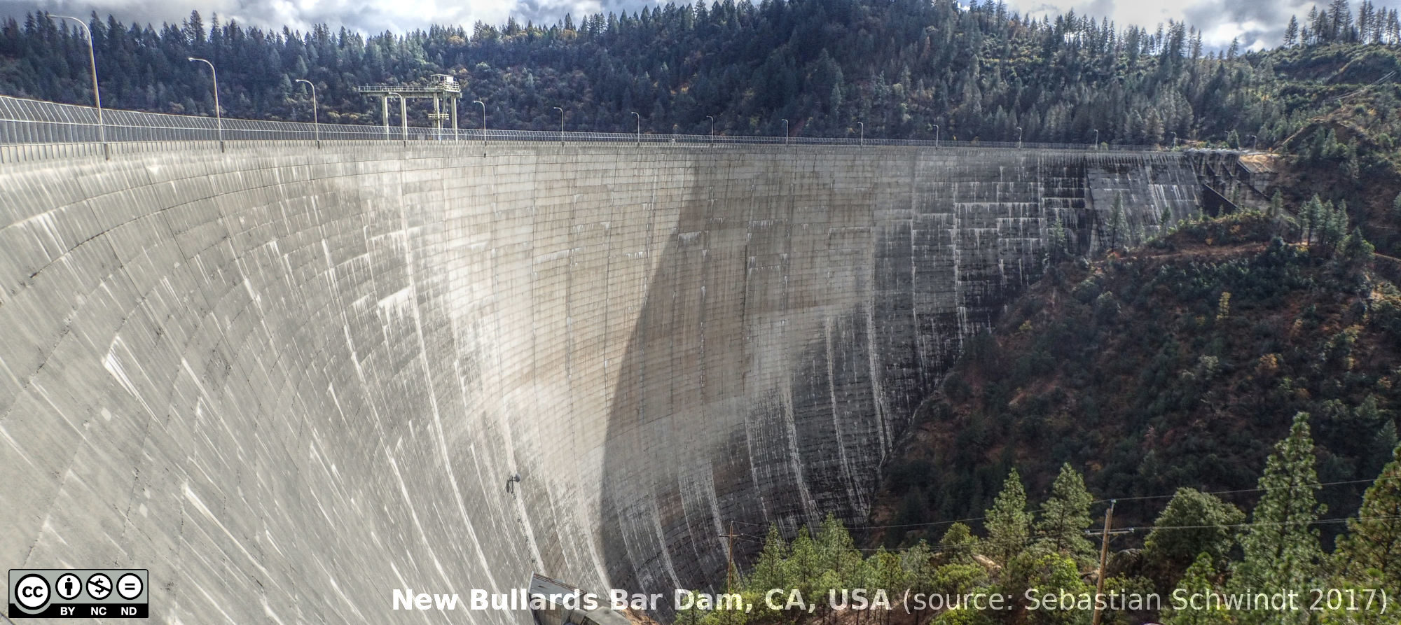
Figure 1:Neuer Bullards Bar Dam in Kalifornien, USA (Quelle: Sebastian Schwindt 2017).
Theorie
Saisonale Speicherreservoirs speichern Wasser in nassen Monaten (z. B. Monsun oder regnerische Winter im mediterranen Klima), um eine ausreichende Trinkwasser- und Agrarversorgung in trockenen Monaten zu gewährleisten. Dazu sind enorme Speichervolumina notwendig, die oft 1.000.000 m überschreiten.
The necessary storage volume is determined from historical inflow measurements and target discharge volumes (e.g., agriculture, drinking water, hydropower, or ecological residual water quantities). The sequent peak algorithm Potter, 1977 based on Rippl (1883) is a decades-old procedure for determining the necessary seasonal storage volume based on a storage volume curve (SD curve). The below figure shows an exemplary curve with volume peaks (local maxima) approximately every 6 months and local volume minima between the peaks. The volume between the last local maximum and the lowest following local minimum determines the required storage volume (see the bright-blue line in the figure).
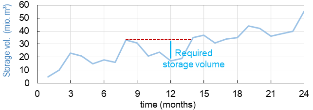
Figure 2:Schema des sequenten Peak-Algorithmus.
Der sequente Peak-Algorithmus wiederholt diese Berechnung über mehrere Jahre und das höchste beobachtete Volumen bestimmt das erforderliche Volumen.
In this exercise, we use daily flow measurements from Vanilla River (in Vanilla-arid country with monsoon periods) and target outflow volumes to supply farmers and the population of Vanilla-arid country with sufficient water during the dry seasons. This exercise guides you through loading the daily discharge data, creating the monthly (storage) curve, and calculating the required storage volume.
Vorverarbeitung von Durchflussdaten
Die täglichen Flussdaten des Vanilla-Flusses sind von 1979 bis 2001 in Form von .csv-Dateien (flowsfolder]) verfügbar.
Schreibe eine Funktion zum Lesen von Flussdaten
The function will loop over the csv file names and append the file contents to a dictionary of numpy arrays. Make sure to import numpy as np, import os, and import glob.
Choose a function name (e.g.,
def read_data(args):) and use the following input arguments:directory: String eines Pfades zu Dateienfn_prefix: String des Dateipräfixes, um Dict-Keys von einem Dateinamen zu entfernenfn_suffix: String des Dateisuffix, um Dict-Keys von einem Dateinamen zu entfernenftype: String von Dateiendungendelimiter: String des Spaltentrenners
In the function, test if the provided directory ends on
"/"or"\\"with
directory.endswith("/") or directory.endswith("\\")
and read all files that end withftype(we will useftype="csv"here) with thegloblibrary:if True:get the the csv (ftype) file list as
file_list = glob.glob(directory + "*." + ftype.strip(".").if False:get the the csv (ftype) file list as
file_list = glob.glob(directory + "/*." + ftype.strip(".")(the difference is only one powerful"/"sign).
Erstellen Sie das Void-Wörterbuch, das den Dateiinhalt als numpy-Arrays enthält:
file_content_dict = {}Loop over all files in the file list with
for file in file_list:Generate a key for
file_content_dict:Trennen Sie den Dateinamen von
file(Verzeichnis + Dateiname + Dateiendeftype) mitraw_file_name = file.split("/")[-1].split("\\")[-1].split(".csv")[0]Strip the user-defined
fn_prefixandfn_suffixstrings from the raw file name and use atry:statement to convert the remaining characters to a numeric value:int(raw_file_name.strip(fn_prefix).strip(fn_suffix)*Note: We will use later on
fn_prefix="daily_flows_andfn_suffix=""to turn the year contained in the csv file names to the key infile_content_dict.Verwenden Sie
except ValueError:für den Fall, dass der verbleibende String nicht inintkonvertiert werden kann:dict_key = raw_file_name.strip(fn_prefix).strip(fn_suffix)(wenn alles gut codiert ist, muss das Skript später nicht in diese Ausnahmeerklärung springen).
Öffnen Sie das
file(Vollverzeichnis) als Datei:with open(file, mode="r") as f:Read the file content with
f_content = f.read(). The string variablef_contentwill look similar to something like";0;0;0;0;0;0;0;0;0;2.1;0;0\n;0...".
Um die Anzahl der (gültigen) Zeilen in jeder Datei zu erhalten
rows = f_content.strip("\n").split("\n").__len__()Um die Anzahl der (gültigen) Spalten in jeder Datei zu erhalten
cols = f_content.strip("\n").split("\n")[0].strip(delimiter).split(delimiter).__len__()Jetzt können wir ein void *numpy * Array der Größe (Form) erstellen, das der Anzahl der gültigen Zeilen und Spalten in jeder Datei entspricht:
data_array = np.empty((rows, cols), dtype=np.float32)Warum verwenden wir nicht direkt
np.empty((31, 12), obwohl die Form aller Dateien gleich ist?
Wir möchten eine allgemein gültige Funktion schreiben und die beiden Zeilen zur Ableitung der gültigen Anzahl von Zeilen und Spalten erledigen den Generalisierungsjob.Next, we need to parse the values of every line and append them to the until now void
data_array. Therefore, we splitf_contentinto its lines withsplit("\n)and use a for loop:for iteration, line in enumerate(f_content.strip("\n").split("\n"):.
Create an empty list to store line dataline_data = [].
In another for loop, strip and split the line by the user-defineddelimiter(recall: we will usedelimiter=";")for e in line.strip(delimiter).split(delimiter):. In the e-for loop,try:to appendeas a float numberline_data.append(np.float32(e)and useexcept ValueError:toline_data.append(np.nan)(i.e., append a not-a-number value that we will need because not all months have 31 days).
End the e-for loop by back-indenting to thefor iteration, line in ...loop and appending theline_datalist as a numpy array todata_array:data_array[iteration] = np.array(line_data)Back in the
with open(file, ...statement (use correct indentation level!), updatefile_content_dictwith the above-founddict_keyand thedata_arrayof thefile as f:file_content_dict.update({dict_key: data_array})Zurück auf der Ebene der Funktion (
def read_data(...):- achten Sie auf die richtige Einrückung!),return file_content_dict
Überprüfen Sie, ob die Funktion wie gewünscht funktioniert, und folgen Sie der Anweisung im Abschnitt Drehen Sie Skript stand-alone, um eine if __name__ == "__main__":-Anweisung am Ende der Datei zu implementieren. Daher sollte das Skript dem folgenden Codeblock ähnlich aussehen:
import glob
import os
import numpy as np


def read_data(directory="", fn_prefix="", fn_suffix="", ftype="csv", delimiter=","):
    # see above


if __name__ == "__main__":
    # LOAD DATA
    file_directory = os.path.abspath("") + "\\flows\\"
    daily_flow_dict = read_data(directory=file_directory, ftype="csv",
                                fn_prefix="daily_flows_", fn_suffix="",
                                delimiter=";")
    print(daily_flow_dict[1995])
Das Ausführen des Skripts gibt den numpy.array der täglichen Durchschnittsströme für das Jahr 1995 zurück:
    [[  0.    0.    0.    0.    0.    0.    0.    0.    0.    0.    0.    0. ]
     [  0.    0.    0.    0.    0.    0.    0.    0.    0.    0.    0.    0. ]
     [  0.    0.    0.    0.    0.    0.    0.    0.    0.    0.    0.    0. ]
     [  0.    4.    0.   14.2   0.    0.    0.   81.7   0.    0.    0.    0. ]
     [  0.    0.    0.    0.    0.    0.    0.    0.    0.    0.    0.    0. ]
     [  0.    0.    0.    0.    0.    0.    0.    0.    0.    0.   19.7   0. ]
     [  0.    0.   19.8   0.    0.    0.    0.    0.    0.    0.    0.    0. ]
     [  0.    0.    4.8   0.    0.    0.   77.2   0.    0.    0.    0.    0. ]
     [  0.    0.    0.    0.    0.    0.    0.    0.    0.    0.    0.    0. ]
     [  0.    0.    0.    0.    0.    0.    0.    0.    0.    0.    0.    0. ]
     [  0.    0.    0.    0.    0.    0.    0.    0.    0.    0.    0.    0. ]
     [  0.    0.    0.    0.   10.2   0.    0.    0.    0.    0.    0.   12. ]
     [  0.    0.    0.    0.    0.    0.    0.    0.    0.    0.    0.  671.8]
     [  0.    0.    0.    0.    0.    0.    0.    0.    0.    0.    0.    0. ]
     [  4.6   0.    0.    0.    0.    0.    0.    0.    0.    0.    0.    0. ]
     [  0.    0.    0.    0.    0.    0.    0.   34.2   0.    0.    0.    0. ]
     [  0.    0.    0.    6.3   0.    0.    0.    0.    0.    0.    0.    0. ]
     [  0.    0.    0.    0.    0.    0.    0.    0.    0.    0.    0.    0. ]
     [  0.    0.    0.    0.    0.    0.    0.    0.    0.   25.3   0.    0. ]
     [  0.    0.    0.    0.    0.    0.    0.    0.    0.    0.    0.    0. ]
     [  0.    0.    0.    0.    0.    0.    0.    0.    0.    0.    0.    0. ]
     [  0.    0.    0.    0.    0.    0.    0.    0.    0.    0.    0.    0. ]
     [  0.    0.    0.    0.    0.    5.    0.    0.    0.    0.    0.    0. ]
     [  0.    0.    0.    0.    0.    0.    0.    0.    0.    0.    0.    0. ]
     [  0.    0.    0.    0.    0.    0.    0.    0.    0.    0.    0.    0. ]
     [  0.    0.    0.    0.    0.    0.   98.7   0.    0.    0.    0.    0. ]
     [  0.    0.    0.    0.    0.    0.    0.    0.   22.1   0.    0.    0. ]
     [  0.    0.    0.    0.    0.    0.    0.    0.    0.    0.    0.    0. ]
     [  0.    nan   0.    0.    0.    0.    0.    0.    0.    0.    0.    0. ]
     [  0.    nan   0.    0.    0.    0.    0.    0.    0.    0.    0.    0. ]
     [  0.    nan   0.    nan   0.    nan   0.    0.    nan   0.    nan   0. ]]
Tagesflüsse in Monatsvolumina umrechnen
The sequent peak algorithm takes monthly flow volumes, which corresponds to the sum of daily average discharge multiplied with the duration of one day (e.g, 11.0 m/s 24 h/d 3600 s/h). Reading the flow data as above shown results in annual flow tables (average daily flows in m/s) with the numpy.arrays of the shape 31x12 arrays (matrices) for every year. We want to get the column sums and multiply the sum with 24 h/d 3600 s/h. Because the monthly volumes are in the order of million cubic meters (CMS), dividing the monthly sums by 10**6 will simplify the representation of numbers.
Schreibe eine Funktion (z.B. def daily2monthly(daily_flow_series)), um die Umwandlung von täglichen durchschnittlichen Flussreihen in monatliche Volumen in 10m durchzuführen:
Die Funktion sollte für jeden Wörterbucheintrag (Jahr) der Datenreihe aufgerufen werden. Daher sollte das Eingabeargument
daily_flow_serieseinnumpy.arraymit der Form(31, 12)sein.Um spaltenweise (monatliche) Statistiken zu erhalten, transponieren Sie das Eingabefeld:
daily_flow_series = np.transpose(daily_flow_series)Create a void list to store monthly flow values:
monthly_stats = []Loop over the row of the (transposed)
daily_flow_seriesand append the sum multiplied by24 * 3600 / 10**6tomonthly_stats
for daily_flows_per_month in daily_flow_series:
    monthly_stats.append(np.nansum(daily_flows_per_month * 24 * 3600) / 10**6)
Zurück
monthly_statsalsnumpy.array:
return np.array(monthly_stats)Mit einer for-Schleife können wir nun die monatlichen Volumina ähnlich den täglichen Flüssen in ein Wörterbuch schreiben, das wir jeweils um ein Jahr innerhalb der if __name__ == "__main__"-Anweisung erweitern:
import ...


def read_data(directory="", fn_prefix="", fn_suffix="", ftype="csv", delimiter=","):
    # see above section


def daily2monthly(daily_flow_series):
    # see above descriptions


if __name__ == "__main__":
    # LOAD DATA
    ...
    # CONVERT DAILY TO MONTHLY DATA
    monthly_vol_dict = {}
    for year, flow_array in daily_flow_dict.items():
        monthly_vol_dict.update({year: daily2monthly(flow_array)})
Sequenzierter Spitzenalgorithmus
Mit den oben genannten Routinen zum Lesen der Flussdaten haben wir monatliche Zuflussvolumina in Millionen m (gespeichert in monthly_vol_dict) abgeleitet. Für die Bewässerung und Trinkwasserversorgung will das Vanilla-aride Land folgendes Jahresvolumen aus dem Reservoir entnehmen:
| Monat | Jan | Feb | Mar | Apr | May | Jun | Jul | Aug | Sep | Oct | Nov | Dec |--------------------------------------------------------------------------------------------------------------------------------------------------------------------------------------------------------------------------------------------------------------- | Vol. (10 m) | 1.5 | 1.5 | 1.5 | 2 | 4 | 4 | 5 | 5 | 3 | 2 | 1.5 |
Following the scheme of inflow volumes we can create a numpy.array for the monthly outflow volumes .
monthly_supply = np.array([1.5, 1.5, 1.5, 2.0, 4.0, 4.0, 4.0, 5.0, 5.0, 3.0, 2.0, 1.5])Speichervolumen und Differenz (SD-Zeilen) Kurven
The storage volume of the present month is calculated as the result of the water balance from the last month, for example:
= + -
= + - = + + - -
In Summationsnotation können wir schreiben:
Die letzten beiden Begriffe bilden die Speicherdifferenz () Zeile:
Thus, the storage curve as a function of the line is:
Die Summennotation der Speicherkurve als Funktion der -Zeile ermöglicht es uns, die Berechnung in eine einfache def sequent_peak(in_vol_series, out_vol_target):-Funktion zu implementieren.
Die neue def sequent_peak(in_vol_series, out_vol_target):-Funktion muss:
Berechnen Sie die monatlichen Speicherdifferenzen ( - ), zum Beispiel in einer for Schleife über das
in_vol_seriesWörterbuch:
    # create storage-difference SD dictionary
    SD_dict = {}
    for year, monthly_volume in in_vol_series.items():
        # add a new dictionary entry for every year
        SD_dict.update({year: []})
        for month_no, in_vol in enumerate(monthly_volume):
            # append one list entry per month (i.e., In_m - Out_m)
            SD_dict[year].append(in_vol - out_vol_target[month_no])
Verflachen Sie das Wörterbuch zu einer Liste (das hätten wir auch direkt tun können), die der oben definierten -Zeile entspricht:
    SD_line = []
    for year in SD_dict.keys():
        for vol in SD_dict[year]:
            SD_line.append(vol)
Calculate the storage line with
storage_line = np.cumsum(SD_line)Finden Sie lokale Extrema und es gibt zwei (und mehr) Optionen:
Verwenden Sie
from scipy.signal import argrelextremaund erhalten Sie die Indizes (Positionen von) lokalen Extrema und deren Wert vonstorage_line:
seas_max_index = np.array(argrelextrema(storage_line, np.greater, order=12)[0])
seas_min_index = np.array(argrelextrema(storage_line, np.less, order=12)[0])
seas_max_vol = np.take(storage_line, seas_max_index)
seas_min_vol = np.take(storage_line, seas_min_index)
Schreibe zwei Funktionen, die nacheinander lokale Maxima und dann lokale Minima zwischen den Extrema finden (Kurs Hausaufgaben) ODER verwenden Sie
from scipy.signal import find_peaks, um die Indizes (Positionen) zu finden - überlegen Sie, einefind_seasonal_extrema(storage_line)-Funktion zu schreiben.
Stellen Sie sicher, dass die Kurven und Extrema korrekt sind, indem Sie die bereitgestellte
plot_storage_curve-Kurve in Ihr Skript kopieren (verfügbar im Übungsrepository]) und wie folgt verwenden:
plot_storage_curve(storage_line, seas_min_index, seas_max_index, seas_min_vol, seas_max_vol)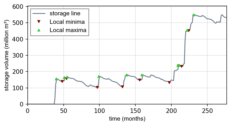
Figure 3:Speicherdifferenzkurve (SD).
Berechnen des erforderlichen Speichervolumens
The required storage volume corresponds to the largest difference between a local maximum and its consecutive lowest local minimum. Therefore, add the following lines to the sequent_peak function:
    required_volume = 0.0
    for i, vol in enumerate(list(seas_max_vol):
        try:
            if (vol - seas_min_vol[i]) > required_volume:
                required_volume = vol - seas_min_vol[i]
        except IndexError:
            print("Reached end of storage line.")
Schließen Sie die Funktion sequent_peak mit return required_volume
Call sequent Peak Algorithmus
Wenn alle erforderlichen Funktionen geschrieben sind, besteht die letzte Aufgabe darin, die Funktionen in der if __name__ == "__main__"-Anweisung aufzurufen:
import ...


def read_data(directory="", fn_prefix="", fn_suffix="", ftype="csv", delimiter=","):
    # see above section


def daily2monthly(daily_flow_series):
    # see above section


def sequent_peak(in_vol_series, out_vol_target):
    # see above descriptions

if __name__ == "__main__":
    # LOAD DATA
    ...
    # CONVERT DAILY TO MONTHLY DATA
    ...
    # MAKE ARRAY OF MONTHLY SUPPLY VOLUMES (IN MILLION CMS)
    monthly_supply = np.array([1.5, 1.5, 1.5, 2.0, 4.0, 4.0, 4.0, 5.0, 5.0, 3.0, 2.0, 1.5])
    # GET REQUIRED STORAGE VOLUME FROM SEQUENT PEAK ALGORITHM
    required_storage = sequent_peak(in_vol_series=monthly_vol_dict, out_vol_target=monthly_supply)
print("The required storage volume is %0.2f million CMS." % required_storage)Schlussbemerkungen
Die Verwendung des sequenten Peak-Algorithmus (auch bekannt als Rippl-Methode, aufgrund seines ursprünglichen Autors) hat sich weiterentwickelt und wurde in anspruchsvolle Algorithmen zur Steuerung des Speichervolumens mit Prädiktormodellen (statistisch und / oder numerisch) implementiert.
Am Ende gibt es mehrere Algorithmen und Möglichkeiten, sie zu codieren. Viele Faktoren (z. B. Gelände oder Klimazone) bestimmen, ob eine saisonale Lagerung möglich oder notwendig ist. Bei der Bestimmung des Speichervolumens dürfen soziale und ökologische Aspekte nicht vernachlässigt werden. Jedes zurückgehaltene Sedimentkorn fehlt in flussabwärts gelegenen Abschnitten, jeder Fisch, der nicht mehr wandern kann, erleidet einen Verlust an Lebensraum, und vor allem jeder Bewohner, der wirtschaftliche Verluste erleidet oder sogar gezwungen ist, sich wegen des Damms umzusiedeln, muss vermieden oder angemessen entschädigt werden.
- Potter, K. W. (1977). Sequent Peak Procedure: Minimum Reservoir Capacity Subject to Constraint on Final Storage. JAWRA Journal of the American Water Resources Association, 13(3), 521–528. 10.1111/j.1752-1688.1977.tb05564.x
- Rippl, W. (1883). The capacity of storage-reservoirs for water-slpply. (including plate). Minutes of the Proceedings of the Institution of Civil Engineers, 71(1883), 270–278. 10.1680/imotp.1883.21797