Machen Sie sich bereit, indem Sie das Übungsrepository klonen:
git clone https://github.com/Ecohydraulics/Exercise-FloodReturn.git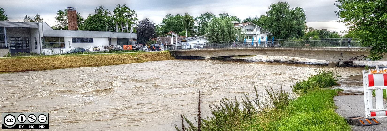
Figure 1:Überschwemmung am Mangfall in Bayern (Quelle: KSS 2020).
Terminologie
Die Hochwasserfrequenzanalyse verwendet eine Reihe von Entladungsdaten (z. B. von einer Messstation) und wertet die Eintrittswahrscheinlichkeit einer bestimmten Entladung aus. Die Ereigniswahrscheinlichkeit definiert somit die Häufigkeit einer Entladung, was aus zwei Gründen wichtig ist:
Überwassersicherheit: Viele rechtliche Rahmen verwenden ein **wiederkehrendes Intervall ** (dh eine Rückkehrzeit oder Häufigkeit in Einheiten von Jahren), um Sicherheitsniveaus zu definieren, die Gebäude und Infrastruktur erfüllen müssen.
Ökohydraulik: Insbesondere in trockenen Gebieten ist es wichtig zu wissen, wie lange bestimmte Ableitungen unter bestimmten Werten liegen, wo viele aquatische Lebensräume möglicherweise nicht tief genug, zu heiß oder vom Hauptkanal getrennt sind. Daher möchten wir die Überschreitungswahrscheinlichkeit einer bestimmten Entlastung wissen.
Die Beziehung zwischen der Überschreitungswahrscheinlichkeit und dem Rezidivintervall ergibt sich aus der Definition beider Begriffe:
Die Überschreitungswahrscheinlichkeit ist die Wahrscheinlichkeit eines Ereignisses einer bestimmten Größenordnung (in m/s oder CFS) oder höher.
Das Rezidivintervall ist die Umkehrung der Überschreitungswahrscheinlichkeit und drückt die durchschnittliche Rückgabedauer eines Ereignisses einer bestimmten Größe in Zeiteinheiten aus.
Das Berechnungskonzept der Renditeperiode macht zwei elementare Annahmen. Zunächst wird angenommen, dass die einzelnen Strömungsereignisse einen stationären Peak aufweisen. Zweitens wird die statistische Unabhängigkeit einzelner Ereignisse angenommen. Die Annahme der statistischen Unabhängigkeit bedeutet, dass in diesem Jahr eine 100-jährige Flut mit der gleichen Wahrscheinlichkeit auftritt wie im nächsten Jahr, unabhängig davon, ob in diesem Jahr tatsächlich eine 100-jährige Flut aufgetreten ist oder nicht. Für jedes gegebene Jahr beträgt die Wahrscheinlichkeit, dass eine 100-jährige Flut auftritt, 1/100 (oder 1/50 für eine 50-jährige Flut und so weiter).
Die Wahrscheinlichkeit einer 100-jährigen Überschwemmung beträgt in 100 Jahren 63 %
As engineers we often want to know how likely it is that a 100-year flood will occur within the next 2, 5, 10, ... or 100 years (i.e., what are the likely costs of flood damage associated with a 100-year flood?). The answer to that question is “the opposite likelihood of no 100-year flood occurring in the next 2, 5, or 10 years”. Mathematically that means the annual occurrence probability of an event with a recurrence interval years over an observation period of years is:
Table 1 zeigt Lösungen für die Wahrscheinlichkeitsfunktion für Beobachtungszeiträume von 2, 5, 10 und 100 Jahren sowie Rezidivintervalle von 10, 50 und 100 Jahren.
Table 1:Solutions to the probability function for selected observation periods .
=2 | =5 | =10 | =100 | |
|---|---|---|---|---|
=10 | 19,00 % | 40,95% | 65,13% | 100,00 % |
=50 | 3,96% | 9,61% | 18,29% | 86,74% |
=100 | 1,99 % | 4,90 % | 9,56% | 63,40 % |
Besuchen Sie die USGS Wasserwissenschaftsschule, um mehr über das Wiederauftreten von Überschwemmungen (und Dürren) zu erfahren.
Löschen von Daten
Datenquellen herunterladen
Flussdaten können von Messstationen abgerufen werden. In Deutschland bietet das [Gewässerkundliches Jahrbuch]](http://www.dgj.de/) einen zusammengesetzten Überblick über statistische Daten von Messstationen. Beachten Sie, dass viele Messstationen, wie auch in vielen anderen Ländern, von staatlichen Behörden verwaltet werden und nur ein kleiner Teil der Daten von Bundesinstitutionen verfügbar ist. Zum Beispiel sind Messdaten für Baden-Württemberg beim Landesinstitut für Umwelt, Erhebung und Naturschutz (LUBW) verfügbar geo portal]. Die folgende Liste enthält weitere Quellen für Entladungsdaten rund um den Globus.
Die Bundesanstalt für Gewässerkunde BfG betreibt das Global Runoff Data Centre GRDC] für die Weltorganisation für Meteorologie WMO, um weltweit Flussabflussdaten bereitzustellen. Die Download-Plattform der GRDC ist in Form eines interaktiven web-GIS] verfügbar. Um die Daten zu erhalten, gehen Sie zu ihrer Download interface, wählen Sie die gewünschte Station aus, wechseln Sie zur Tabellen-Ansicht (dritte Zeile oben links im Fenster), überprüfen Sie die Station, klicken Sie auf Download und füllen Sie das Formular aus, um die Anfrage zu senden. Sie erhalten eine E-Mail mit einem Download-Link für die angeforderten Daten (warten Sie einige Minuten, bevor Sie auf den Link klicken - die Vorbereitung kann mehr Zeit in Anspruch nehmen als die E-Mail).
Flussdatensätze von alpinen und mittleren Flüssen werden vom Schweizerischen Bundesamt für Umwelt zur Verfügung gestellt hydrologische Datenplattform (für Langzeitbeobachtungen muss auch hier ein Formular ausgefüllt werden).
In den Vereinigten Staaten liefert die National Oceanic and Atmospheric Administration * NOAA* Ableitungsdaten aus der Vergangenheit und Prognosen für Wassereinzugsgebiete in Nordamerika. Zum Beispiel bietet das California Nevada River Forecast Center] Flussprognosen für den Südwesten der Vereinigten Staaten, und historische Daten können über das California Data Exchange Center CDEC] abgerufen werden.
Eine allgemeine US-Schnittstelle zum Laden von Flussdaten und Statistiken ist mit der
hydrofunctionsPython library, die vom United States Geological Survey USGS bereitgestellt wird, ausgestattet.] Diese Bibliothek ermöglicht es, direkt Messdaten und Statistiken basierend auf einer Stream-Messe-ID abzurufen. Zum Beispieloutput = hydrofunctions.peaks("01541200")Um
hydrofunctionsin einer conda Umgebung zu installieren, geben Sieconda install -c conda-forge hydrofunctionsin Anaconda Prompt ein.Anwendungsbeispiel:
import hydrofunctions as hf
hf.draw_map()` # only runs in JupyterLab
Ladedaten mit pandas
Create a new Python file (e.g., discharge_analysis.py) and import pandas as pd at the beginning. Read the provided flow data series file "daily-flow-series.csv" with pd.read_csv.
The header (column names) is in row 36, but we do not use the column names from the csv file and overwrite them with the names argument ("Date" and "Q (CMS)" (for Cubic Meters per Second)). Alternatively, we could use the skiprows argument to indicate where the data content starts in the file.
With sep=";", we indicate that columns are separated by a semicolon. The usecols=[0, 2] argument specifies that we only want to read columns 0 (date) and 2 (discharge) because the information content of column 1 (time) is not relevant for daily discharge. The parse_dates=[0] argument lets pandas know that column 0 contains date-formatted values. Alternatively, we could use a dtype={"Date": ... } dictionary to specify the data formats of columns. However, using dtype would require importing datetime and induce unnecessary complexity. In addition, the index_col argument defines the column indices, which need to have a date format for the later analyses. In addition, use the optional keyword argument encoding="latin1" because the provided data file contains some special characters that cannot be recognized with the standard utf-8 encoding.
import pandas as pd
df = pd.read_csv("flow-data/daily-flow-series.csv",
                 header=36,
                 sep=";",
                 names=["Date", "Q (CMS)"],
                 usecols=[0, 2],
                 parse_dates=[0],
                 index_col="Date")
Hat alles funktioniert? Überprüfen Sie das geladene data_series mit print(data_series.head())
If your CSV file has special characters (e.g. 3), you may need to use the optional keyword argument encoding="latin1" because some special characters cannot be recognized with the standard utf-8 encoding.
Geben Sie die Daten
Plotting data is not the focus of this exercise and for this reason, there is a ready-to-use function available in the plot_discharge.py script. Make sure that the plot_discharge.py is in the same directory as the above discharge_analysis.py Python script (recall how to load Pakete, Module und Bibliotheken). Use the plot_discharge function in plot_discharge.py as follows:
from plot_discharge import plot_discharge
plot_discharge(df.index, df["Q (CMS)"], title="Daily Flows 1826 - 2016")
On a side note, plot_discharge uses the Matplotlib library.
Baureihe der jährlichen Höchstentladung
Flood event recurrence intervals result from statistics of the annual maximum discharge. Therefore, use pandas’ resample function to find annual maximum values. The resample function requires the definition of a DateTimeIndex, which we already implemented by using the index_col argument when we loaded the data. The first (and only required) argument for the resample function is the rule defining the length of the time frame to which re-sampling applies. Here, we use "A" for annual statistics. For using bi-annual or 5-year periods, we could use the rule "5A". More rules can be found at the pandas docs.
In addition, we use the argument kind=period, because we are only interested in the year in which the discharge occurred. Finally, we apply .max() to run maximum statistics on the data frame. Since the re-sampled dataframe is again a dataframe, all dataframe methods can also be applied to it. That is, instead of max() we can as well use min(), sum(), median(), mean() and so on (see pandas dataframe methods).
annual_max_df = df.resample(rule="A", kind="period").max()Because we use kind="period", the row indices of annual_max_df correspond to time periods of years. For instance, the row index 1826 corresponds to the period 1826-01-01 through 1826-12-31. However, we need integer numbers of years rather than periods for the calculation of return periods. To get integer formats of years, we transfer the year of each period into a new column of the data frame and reset the row indices. Resetting the row indices to default integer indices through (drop=True) is not absolutely necessary, but serves the physical correctness of the data frame. The argument inplace=True replaces the indices inside annual_max_df (otherwise, we needed to write annual_max_df = annual_max_df.reset_index(drop=True)).
annual_max_df["year"] = annual_max_df.index.year
annual_max_df.reset_index(inplace=True, drop=True)
print(annual_max_df.head()
Optional zeichnen Sie die jährlichen Maxima mit:
plot_discharge(annual_max_df["year"], annual_max_df["Q (CMS)"], title="Annual Flows 1826 - 2016")Berechnung der Überschreitungswahrscheinlichkeit und Wiederauftretensintervalle
Die Überschreitungswahrscheinlichkeit eines bestimmten Ereignisses innerhalb des Beobachtungszeitraums ist:
wo
ist die Gesamtzahl der Beobachtungsjahre und
ist der Rank der Veranstaltung.
Um die Ereignisse einzuordnen, müssen wir zuerst den maximalen jährlichen Entladedatenrahmen (annual_max_df) nach dem kleinsten bis größten Entladewert (und nicht nach der Zeit) sortieren:
annual_max_df_sorted = annual_max_df.sort_values(by="Q (CMS)")Then, we derive the number of observations (n = annual_max_df_sorted.shape[0]) and add a "rank" column, in which we simply enumerate the rows using the range method.
n = annual_max_df_sorted.shape[0]
annual_max_df_sorted.insert(0, "rank", range(1, 1 + n)
Jetzt haben wir alle Zutaten, um die Wahrscheinlichkeit jedes Ereignisses mit den oben gezeigten -formula.
zu berechnen.
annual_max_df_sorted["pr"] = (n - annual_max_df_sorted["rank"] + 1) / (n + 1)Das Rezidivintervall (hier: Rückgabezeit in Jahren) ist die Umkehrung der Überschreitungswahrscheinlichkeit und wir können es dem Datenrahmen hinzufügen mit:
annual_max_df_sorted["return-period"] = 1 / annual_max_df_sorted["pr"]Überprüfen Sie die resultierende höchste Entladung und ihre Rückgabefrist:
print(annual_max_df_sorted.tail()Plot the resulting probability and return curves with the plot functions provided in the plot_result.py Python script:
plot_q_freq(annual_max_df_sorted)
plot_q_return_period(annual_max_df_sorted)Außerhalb der Box
Das hier gezeigte Verfahren ist lediglich eine Interpolation. Für die Extrapolation von Rückkehrperioden über die Länge des Beobachtungszeitraums hinaus (z. B. für Extremereignisse wie eine 1000-jährige Flut) ist ein Vorhersagemodell erforderlich (z. B. Gumbel-Extrapolation).
Schließlich gibt es bereits Software, die Rückgabezeiten berechnet, frei verfügbar im U.S. Army Corps of Engineers Hydrologic Engineering Center (HEC) U.S. Army Corps of Engineeers, 2016: HEC-SPP]. HEC-SPP ermöglicht die Berechnung von Flow-Event-Frequenzen und Rückkehrperioden nach US-Standards. Wenn sie also nicht in oder für die vereinigten staaten arbeiten, möchten sie vielleicht immer noch ihren code bereit haben. Darüber hinaus erfordert HEC-SPP eine Vorverarbeitung der Entladedaten (d.h. es funktioniert nur mit jährlichen Maxima).
- U.S. Army Corps of Engineeers. (2016). Hydrologic Engineering Centers River Analysis System (HEC-RAS). U.S. Army Corps of Engineeers (USACE). http://www.hec.usace.army.mil/software/hec-ras/