Friction (Roughness) Zones
Similar to the assignment of multiple friction coefficient values to multiple model regions featured in the BASEMENT tutorial, Telemac2d provides routines for domain-wise (i.e., zonal) friction area definitions in the geometry (.slf) mesh file. Specifically, if the study domain is characterized by regions of different roughness, it is not sufficient to define global friction through a FRICTION COEFFICIENT keyword in the steering (.cas) file. Defining roughness zones in the mesh (.slf) file requires an additional layer called BOTTOM FRICTION or FRIC_ID on top of the BOTTOM elevation. To this end, roughness values can be defined in a roughness .xyz file created with QGIS (recommended) or Closed Lines .i2s created with BlueKenue (see the meshing section). While QGIS is recommended to delineate roughness zones with correct and possibly precise georeferences, BlueKenue is still required for interpolating the roughness from the .xyz or .i2s file on the .slf file in the last step.
Roughness.XYZ with QGIS (recommended)
The first step for delineating roughness zones in QGIS is to set up the coordinate reference system and save the project, analogous to the QGIS pre-processing tutorial:
Open QGIS, and in the top menu go to Project > Properties.
Activate the CRS tab.
Set the CRS that your basemap / DEM data use; for this example, enter
UTM zone 33Nand select UTM zone 33N (WGS84) (EPSG 32633), which is not a great choice because of its low precision, but it will do the job for this tutorial.Click Apply and OK.
Save the project into a new folder where all files for this tutorial will be stored.
It will be important to avoid overlapping that would lead to ambiguous or missing definitions of regions. Therefore, activate snapping:
Activate the Snapping Toolbar: View > Toolbars > Snapping Toolbar
In the Snapping toolbar > Enable Snapping

Enable snapping for
Vertex, Segment, and Middle of Segments
 .
.Snapping on Intersections
 .
.Self Snapping
 .
.
This tutorial picks up the example from the Telemac QGIS pre-processing tutorial to draw polygons along the breaklines and liquid-boundaries shapefiles. The friction zones are inferred from a Google Satellite basemap and friction attributes are qualitatively estimated, which is just fine for a tutorial. In practice, we strongly recommend performing field surveys on grain size distributions with high-precision differential GPS (DGPS) systems to delineate roughness zones on-site supported by drone imagery.
Delineate Roughness Zone Polygons
The roughness zones can be described by attributes of a polygon shapefile. To create a new polygon shapefile, go to Layer > Create Layer > New Shapefile Layer... (see Fig. 1).
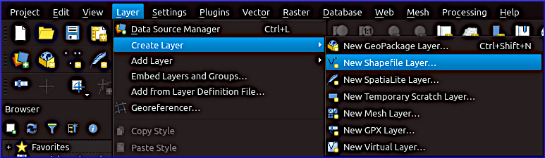
Figure 1:Create a new polygon shapefile.
In the popup window, enter the following definitions:
File name: press on ..., navigate to the project folder, and tap
friction-polygons.File encoding: keep default (sample files use
UTF-8).Geometry type:
PolygonBelow the Additional dimensions (not required), find and click on the CRS button to select the above-defined project coordinate system (example files:
EPSG:32633).Add a New Field:
Name:
dMeanType:
Decimal (double)Length:
10Precision:
5Click Add to Fields List
Add another New Field:
Name:
fricIDType:
Integer (32 bit)Length:
5Click Add to Fields List
Press OK to create the new shapefile.
To follow this tutorial, import the breaklines (download as zip-file) and liquid-boundaries (download as zip-file) shapefiles from the Telemac pre-processing. To draw polygons by editing fiction-polygons.shp along the breaklines and liquid boundaries, highlight fiction-polygons in the Layers panel, and enable editing by clicking on the yellow pen  . Activating Add Polygon Feature and draw polygons by snapping to points of the breaklines and liquid boundaries layers, according to Fig. 2. To finalize each polygon with a right-click on the mouse and enter the
 fricID and dMean values according to Tab. 1 (qualitative grain sizes).
To correct drawing errors use the Vertex Tool  . Finally, save the new polygons (edits of friction-zones.shp) by clicking on the Save Layer Edits
  symbol. Stop (Toggle) Editing by clicking again on the yellow pen symbol.
Alternatively, merge the breaklines and liquid boundaries, and use the Polygonize tool from the Processing Toolbox to convert the merged lines into a polygon shapefile. However, the polygonization will miss some breaklines, which will require editing. Also, the fricID and dMean fields still need to be added through editing.
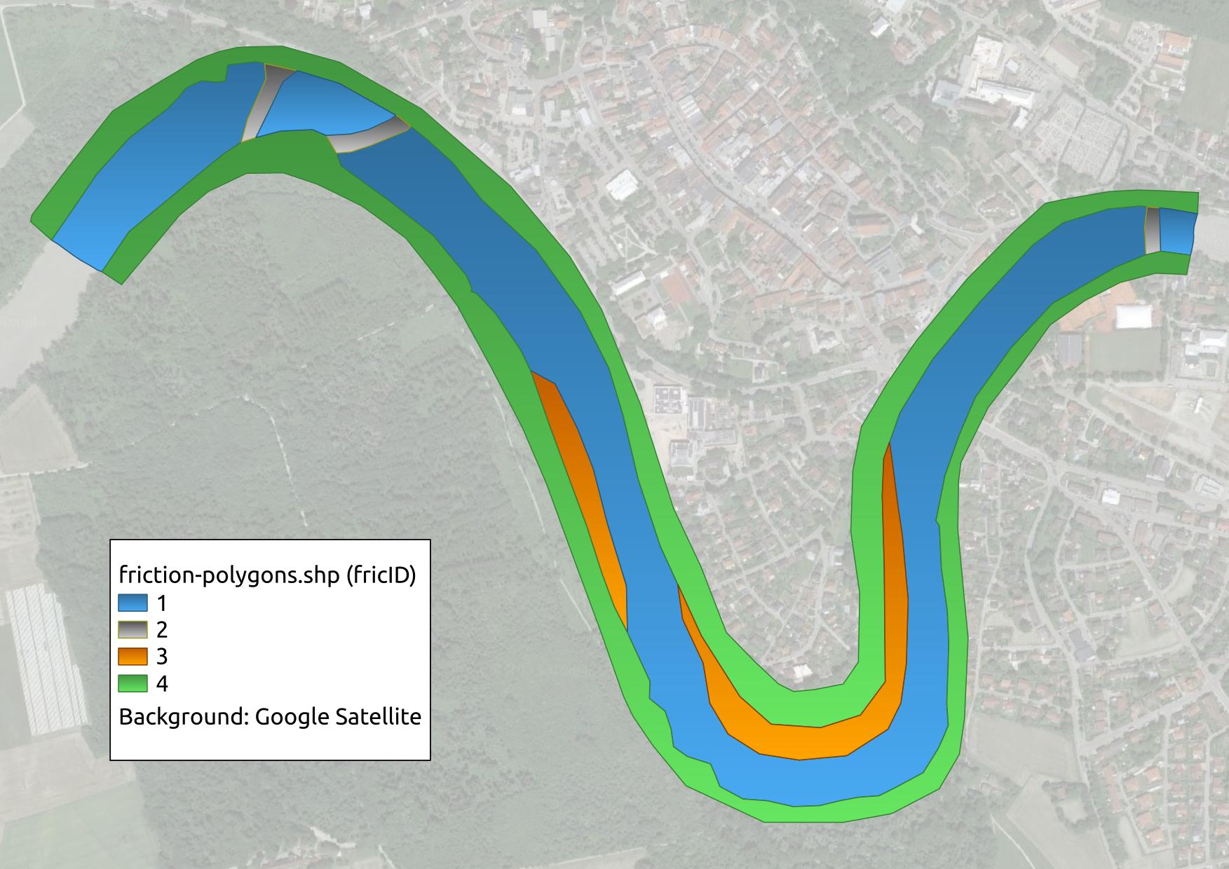
Figure 2:Example for describing roughness (friction) zones with polygons by four friction IDs (fricID) delineating (1) the riverbed, (2) block ramps, (3), gravel bars, and (4) floodplains. Background map: Google (n.d.) satellite imagery.
Table 1:Four exemplary friction zones described by integer fricIDs and mean grain size diameters dMean.
Zone name | Riverbed | Block ramps | Gravel banks | Floodplains |
|---|---|---|---|---|
fricID | 1 | 2 | 3 | 4 |
dMean (m) | 0.080 | 0.300 | 0.032 | 1.000 |
Generate Roughness Points
The next step on the pathway to creating the required XYZ file for assigning friction zones to a selafin geometry file is to generate (random) points inside the above-created polygons. To this end, enter random points inside polygons in the search field of the Processing Toolbox. In the Random Points Inside Polygons popup window (Fig. 3), enter the following:
Input layer:
friction-polygonsSampling strategy:
Points densityPoint count or density:
0.25- use a smaller/larger value for fine/coarse meshes, but beware of potentially very large file sizesMinimum distance between points:
5.0- use a smaller/larger value for fine/coarse meshesRandom points: click on ... and define a target point shapefile name, such as
friction-pts.shpto be stored in the project folder.Click Run to create the points shapefile. This process may take a while depending on the defined point density.
The resulting point shapefile is shown in Fig. 4.
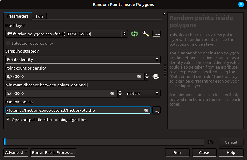
Figure 3:Settings in the Random Points Inside Polygons tool in QGIS. Carefully select the point count or density, which can cause very large output files. The minimum distance field may be used to reduce the number of points.
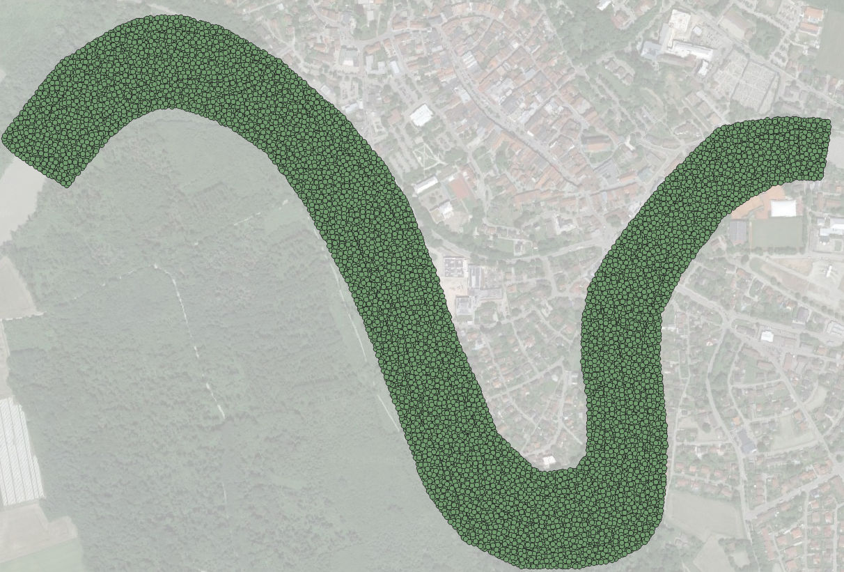
Figure 4:The point shapefile resulting from using the Random Points Inside Polygons tool in QGIS. Background map: Google (n.d.) satellite imagery.
Assign Friction Attributes to Points
Alas, the point generation does not automatically pick up the polygon attributes, which need to be interpolated to the points. Depending on the targeted roughness law for use with Telemac, either the friction IDs or directly roughness coefficients can be added to the attribute table of the friction point shapefile. In this tutorial, a friction coefficient in the form of the Strickler roughness is interpolated and calculated using an empirical formula. A more complex case for calculating roughness values can be found in the BAW’s Donau (Danube) case study (located in HOMETEL/examples/telemac2d/donau/).
The transfer of the dMean and/or fricID attributes of the polygons to the points is essentially an interpolation operation in which QGIS looks at every point and assigns it the dMean and/or fricID attributes of the closest polygon. To this end, click on the Vector top menu > Data Management Tools > Join Attributes by Location (see Fig. 5).
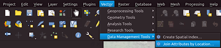
Figure 5:Open the Join Attributes by Location tool in QGIS.
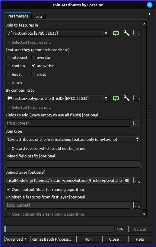
Figure 6:Open the Attribute Table of the friction point table.
In the Join Attributes by Location popup window (Fig. 6) make the following settings:
Join to features in:
friction-ptsFeatures they (geometric predicate): check the
are withinbox, deselect all othersBy comparing to:
friction-polygonsFields to add: click on the ... button to select
fricIDand/ordMeanJoin type:
Take attributes of the first matching feature only (one-to-one)Joined layer: click on the ... button > Save to file > navigate to the project folder > enter a filename, such as
friction-pts-atClick on Run.
The error message No spatial index exists for input layer, performance will be severely degraded can be ignored for this application. Still, to verify any false output, it might be wise to also define the layer Unjoinable features from first layer.
As a result, the friction-pts-at is available in the Layers panel (see Fig. 7).
To convert the mean grain sizes (dMean) into friction values, open the Attribute Table by right-clicking on the friction-pts-at layer in the Layers panel > Open Attribute Table.
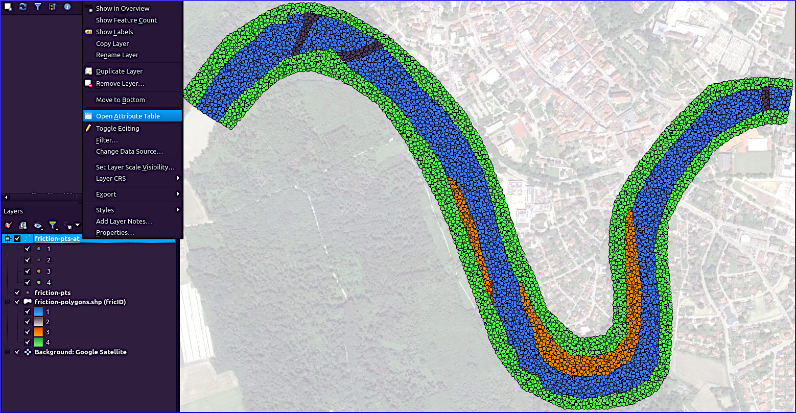
Figure 7:Open the Attribute Table of the friction point shapefile with attribute table. Background map: Google (n.d.) satellite imagery.
Edit the Attribute Table (Fig. 8):
enable editing,
remove unnecessary columns, such as the
idfield, and potentially also thefricIDfield (this showcase will only use thedMeancolumn),open the Field calculator, which we will use in the next step to derive Strickler roughness values.
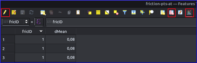
Figure 8:The Attribute Table of the friction-pts-at layer with the highlighted (red rectangles) editing, remove columns, and field calculator buttons (from left to right).
Optional: derive x and y coordinates with the Field Calculator
In the Field Calculator, add the and coordinates to the Attribute Table:
check the box Create a new field
Output field name:
x_coordOutput field type:
Decimal number (real)Output field length:
10and Precision:10Enter a formula by either selecting the x-value from the geometry in the scrollbox or entering directly in the Expression field:
x( @geometry ) Analogously, add the y_coord with:
y( @geometry ) Save the edits in the Attribute Table by clicking on the disk symbol.
According to Meyer-Peter & Müller (1948), the Strickler (1923) roughness (friction) coefficient can be approximated with 26/ based on the grain size , where 90% of the surface sediment grains are smaller. In addition, we will assume that Rickenmann & Recking, 2011. Thus, . To run this calculation, go to the Field Calculator and (see Fig. 7):
check the box Create a new field
Output field name:
k_stOutput field type:
Decimal number (real)Output field length:
3and Precision:2Enter a formula by either selecting
dMeanfromFields and Valuesin the scrollbox or directly entering the equation in the Expression field:
26 / ( ( 2.25 * "dMean" ) ^ ( 1 / 6 ) )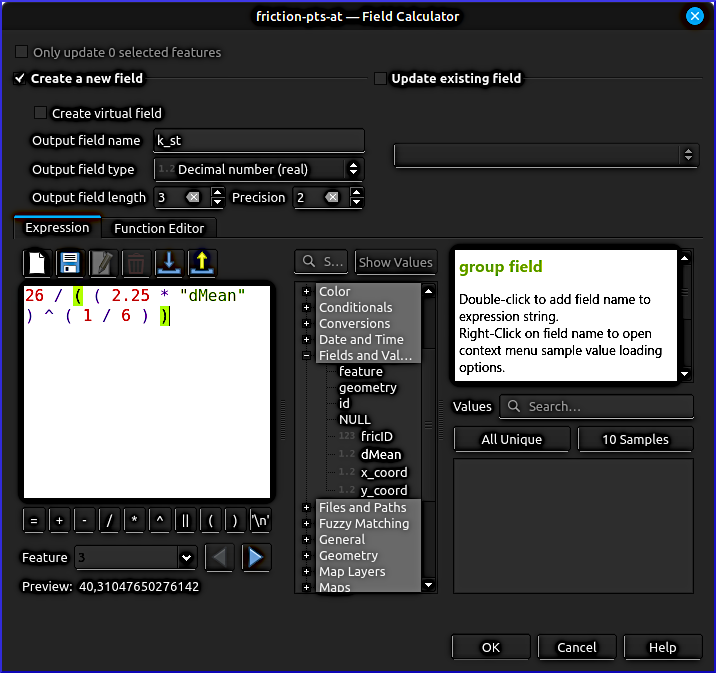
Figure 9:Estimate the Strickler coefficient based on the mean grain size (dMean) with the Field Calculator in QGIS.
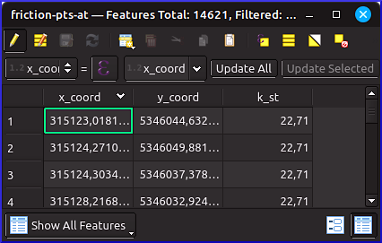
Figure 10:The finalized Attribute Table of the friction-pts-at layer with the optional x and y coordinates, and the estimated Strickler roughness coefficients.
Finally, remove all remaining unnecessary fields from the Attribute Table and save the edits by clicking on the disk symbol, and toggle (i.e., deactivate) editing.
Export Points to XYZ
Start with opening the export dialogue with a right click on the friction-pts-at layer > Export > Save Features As... (Fig. 11).
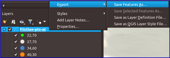
Figure 11:Open the export dialogue with a right click on the friction-pts-at layer > Export > Save Features As...
In the Save Vector Layer as... popup window, make the following settings (Fig. 12):
Format:
Comma Separated Value [CSVFile name: click on ..., navigate to the project folder, and enter
friction-pts.xyzfor file name (press Save).Layer name: keep clear
CRS: make sure the CRS of the friction-pts-at layer is defined (in the showcase
EPSG:32633 - WGS 84 / UTM zone 33N)Encoding: use default (in the showcase
UTF-8)Select all relevant fields, that is, in the showcase, at least
k_st. The optionalx_coordandy_coordfields are only necessary if the geometry is not exported (for whatever reason).Check the Persist layer metadata
Geometry type:
Automatic(mostly default)Scroll down to the Layer Options and:
set the GEOMETRY to
AS_XYset the SEPARATOR to
TAB
Uncheck the Add saved file to map box at the bottom of the window.
Keep all other defaults and click OK.
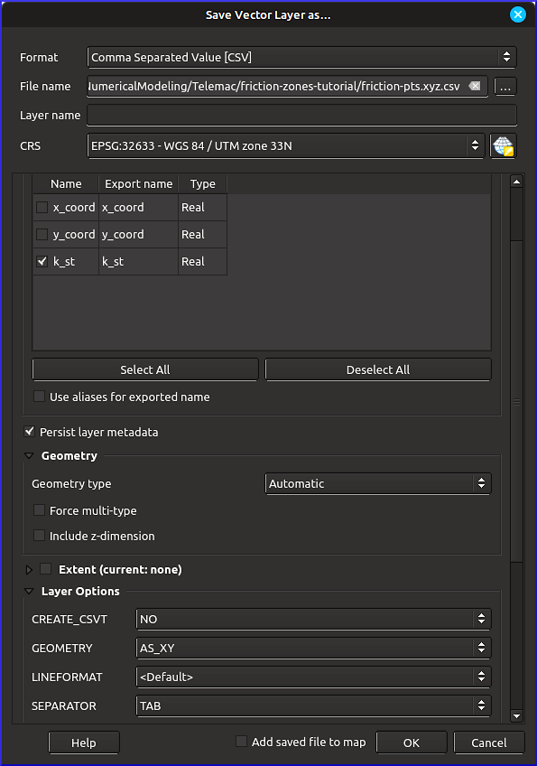
Figure 12:Settings in the Save Vector Layer as... popup window for exporting the friction points to an XYZ (tab-separated CSV) file.
QGIS will have exported the file with a .xyz.csv ending. Rename the file to remove .csv at the end. Verify the correct formatting of the .xyz file by opening it in a text editor (e.g., Notepad++). For instance, if you calculated and exported the x_coord and y_coord fields, and additionally the geometry, the .xyz file will hold two times the coordinates. In this case, import the .xyz file in a spreadsheet editor (i.e., office application), delete the x_coord and y_coord columns, and re-export the file as a tab-separated CSV file. Read more about .xyz file conversion in the QGIS tutorial.
Expand to see the correct header of the showcase friction-pts.xyz file
X Y k_st
315976.648906296  5345616.71281044  40.30
315992.808134594  5345521.13037269  40.30
315983.283370604  5345655.68430873  40.30
315915.433790676  5345754.82689794  40.30
[...]Alternative: Draw Friction Zones in BlueKenue
This procedure is an imprecise alternative to the above-described roughness.xyz creation because of BlueKenue’s weak geospatial referencing capacities, which is why the below instruction box is only provided for completeness.
Unfold to read this non-recommended alternative
Start with creating new closed lines (Fig. 13), similar to polygons delineating roughness zones.
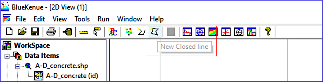
Figure 13:Settings in the Save Vector Layer as... popup window for exporting the friction points to an XYZ (tab-separated CSV) file.
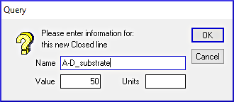
Figure 14:Assign a friction (roughness) value (here: a Strickler roughness of 50) to the delineated area by the closed line.
After drawing a Closed line is finished, press the Esc key and the window shown in Fig. 14 will appear, where a roughness value can be assigned. The exemplary figure assigns a Strickler roughness of 50 in the Value field to a Closed line named A-D_substrate. Continue to assign names to all relevant roughness areas.
Finally, save the Closed line objects as .i2s / .i3s files.
Zonal Friction Mesh (BlueKenue)
This section walks through the interpolation of friction values on an existing selafin (.slf) geometry file. The showcase builds on the .slf file created in the Telemac pre-processing tutorial (download qgismesh.slf). Start with opening BlueKenue and open the selafin .slf file: click on File > Open... > navigate to the directory where the .slf is stored, make sure to select Telemac Selafin File (*.slf), highlight qgismesh.slf, and press Open. Pull the BOTTOM (BOTTOM) layer from the workspace data items to Views > 2D View (1) to verify and visualize the correct import of the mesh (Fig. 15).
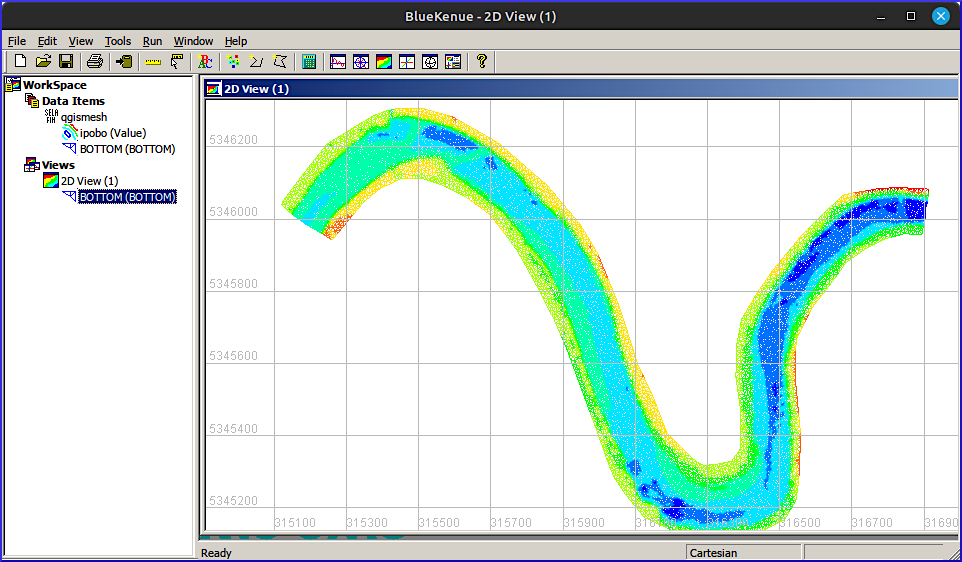
Figure 15:The showcase qgismesh.slf selafin file opened in BlueKenue.
Import Friction Zones
As an alternative to the creation of zonal friction values stored in a .xyz file generated with QGIS, zones can also be directly drawn in BlueKenue through a series of Closed lines. However, because of BlueKenue’s very limited capacities to deal with geospatial references and coordinate systems (CRSs), the preferable option for creating friction zone input is the above-featured application of QGIS.
To open the above-created .xyz file in BlueKenue:
click on File > Open...
navigate to the project folder where the
.xyzis storedmake sure to select All Files (*.*) next to the File name: field
highlight
qgismesh.slf, and press Open.
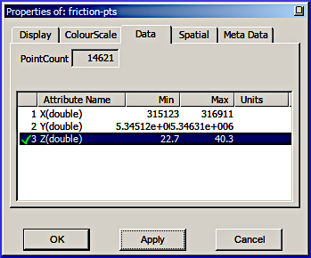
Figure 16:Assign a friction (roughness) value (here: a Strickler roughness of 50) to the delineated area by the closed line.
Ignore the warning message (click OK). To verify and visualize the imported friction values right-click on the friction-pts (X) layer > Properties > go to the Data tab > select Z(double), press Apply. Then, go to the ColourScale tab, press Reset, Apply, and OK.
Verify the correct representation of the friction values by pulling the friction-pts (Z) layer from the workspace data items to Views > 2D View (1) (Fig. 17).
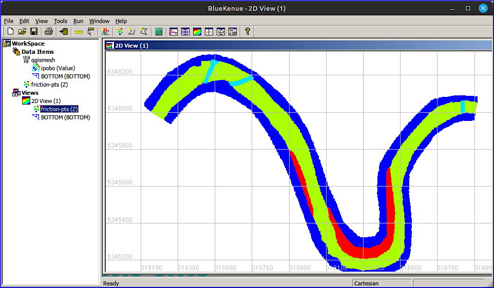
Figure 17:The imported friction-pts.xyz file (created with QGIS) visualized in BlueKenue.
If not yet done, import the Closed lines delineating roughness zones in the form of .i2s / .i3s files.
Interpolate Friction on the Mesh
In BlueKenue, go to File > New > 2D Interpolator, which will occur in the Work Space > Data Items. Drag & drop either the friction-pts .xyz points or the Closed line objects delineating roughness zones on the new 2D Interpolator (see Fig. 18).
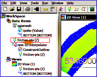
Figure 18:Drag & drop the friction-pts (or closed lines) on a new 2D Interpolator in BlueKenue.
Next, add a new variable to the qgismesh.slf mesh by highlighting the Selafin qgismesh object (in Work Space > Data Items), and right-clicking on it. Click on Add Variable... and enter the following in the popup window (Fig. 19 or Fig. 20), depending on if you are working with friction values (as showcased here with Strickler roughness), or friction IDs (see below):
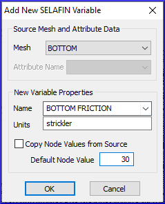
Figure 19:Add a new Variable to the Selafin object for direct friction values.
Mesh:
BOTTOMName:
BOTTOM FRICTION(this example)Units: keep clear (irrelevant field)
Default Node Value:
30(in this example) for a default (Strickler) value to use when no xyz friction points can be found in the vicinity of a mesh node
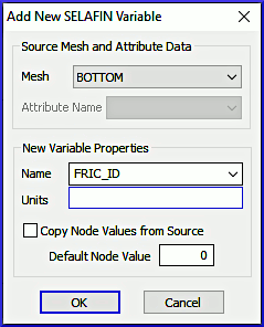
Figure 20:Add a new Variable to the Selafin object for friction IDs.
Mesh:
BOTTOMName:
FRIC_ID(must be entered, cannot be selected from list)Units: keep clear (irrelevant field)
Default Node Value:
0(ID to use when no xyz points can be found in the vicinity of a mesh node)
To interpolate the friction values on the mesh, highlight the new variable variable BOTTOM FRICTION (or FRIC_ID) of the qgismesh object in Work Space > Data Items. The Anonymous Attribute of the new variable can be ignored. To map the new variable onto the mesh:
Highlight the new
BOTTOM FRICTION(orFRIC_ID) mesh variable (in Data Items)Go to Tools > Map Object... (top menu in Fig. 21)
Select the new 2D Interpolator, and click OK, which opens the Processing... popup window
After the processing is completed, click OK.
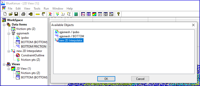
Figure 21:Map the friction value on the new 2D Interpolator in BlueKenue.
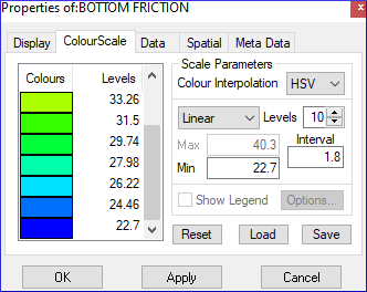
Figure 22:Adjust the color scale for BOTTOM FRICTION.
Verify the correct interpolation:
Define a relevant color scale:
In Work Space > Data Items > qgismesh, right-click on the new BOTTOM FRICTION variable > Properties.
In the properties, go to the ColourScale tab, and use, for example, a Linear scale with
10Levels, a Min of22, and an Interval of1.8. The exemplary minima and interval are good choices for the showcase, but other settings might be preferable for other applications (e.g., prefer Min of0when using Manning’s ).Press Apply > OK.
Drag & drop the BOTTOM FRICTION variable into Views > 2D View (1) to verify the correct interpolation of friction values (e.g., see Fig. 23 for the showcase).
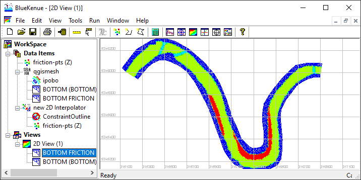
Figure 23:The correctly interpolated new BOTTOM FRICTION variable of the qgismesh.slf mesh.
To save the selafin mesh with interpolated the interpolated friction values, right-click on the qgismesh selafin object > Properties > go to the Meta Data tab, and enter a new Name, for example, qgismesh-friction. Next, highlight the selafin object (e.g., qgismesh-friction) and click on the disk  symbol. If renaming did no take effect on the file name, confirm replacing the existing file.
Telemac Bindings
Implementation in the CAS File
Friction Keywords
The updated qgismesh-friction.slf mesh can be used just like in the steady 2d tutorial, but some keywords need to be modified, even though the BOTTOM FRICTION values assigned in the .slf mesh automatically overwrite the global FRICTION COEFFICIENT keyword in the .cas steering file. However, we need to make Telemac recognize the newly defined BOTTOM FRICTION zones as Strickler roughness type. To this end, change the LAW OF BOTTOM FRICTION to 3 (instead of 4 pointing to Manning’s ), and set the default FRICTION COEFFICIENT to 33 (inverse of = 0.03). The definition of the FRICTION COEFFICIENT is for coherence and is not strictly needed as it will be overwritten by the BOTTOM FRICTION from the .slf mesh.
/ steady2d-zonal-ks.cas steering file
/ ...
/ Friction at the bed
LAW OF BOTTOM FRICTION : 3 / 3-Strickler
FRICTION COEFFICIENT : 33  / will be overwritten by zonal friction values
/ steady2d.cas steering file
/ ...
/ Friction at the bed
LAW OF BOTTOM FRICTION : 4 / 4-Manning
FRICTION COEFFICIENT : 0.03 / Roughness coefficientAdd the letter W to the graphic printouts for writing the friction coefficient to the results file:
/ steady2d-zonal-ks.cas steering file
/ ...
VARIABLES FOR GRAPHIC PRINTOUTS : 'U,V,H,S,Q,W' / add W for friction coefficient
Do you have more than 10 different friction zones?
To increase the number of friction zones recognized by Telemac, set the MAXIMUM NUMBER OF FRICTION DOMAINS keyword, for example, to 20:
/ steady2d-zonal-ks.cas steering file
/ ...
MAXIMUM NUMBER OF FRICTION DOMAINS : 20 / default is 10
Initial Hotstart Conditions (optional)
The following descriptions refer to section 4.1.3 in the Telemac2d manual.
To speed up the simulation, this tutorial re-uses the output of the steady 2d simulation (though, re-created with a printout period of 2500 steps). This type of model initialization is also called hotstart, here, based on the steady results file r2dsteady-t15k.slf, which needs to be defined as PREVIOUS COMPUTATION FILE:
/ steady2d-zonal-ks.cas steering file
/ ...
COMPUTATION CONTINUED : YES
PREVIOUS COMPUTATION FILE : r2dsteady-t15k.slf / results of 35 CMS steady simulation after 15000 timesteps
With the hotstart conditions, the boundaries can be eased to:
/ steady2d-zonal-ks.cas steering file
/ ...
/ Liquid boundaries
PRESCRIBED FLOWRATES  : 35.; 0.
PRESCRIBED ELEVATIONS : 0.; 371.33
For these boundary conditions to take effect, the liquid boundaries file from the steady 2d simulation must be modified:
open boundaries.cli in a text editor
find the
5 5 5(prescribed Q and H) upstream boundary and replace it with4 5 5(prescribed Q only)save and close boundaries.cli
for more information, have a look at the spotlight chapter on boundary conditions
alternatively, download the adapted boundaries.cli here.
Finally, comment out any initial conditions keywords in the .cas steering file, for instance:
/ steady2d-zonal-ks.cas steering file
/ ...
/ INITIAL CONDITIONS : 'ZERO DEPTH'
/ INITIAL DEPTH : 0.005
Run Friction Zone Simulation
Make sure all required files are placed in a simulation folder (e.g., /HOME/modeling/friction-tutorial/), notably:
the qgismesh
-friction .slf mesh with BOTTOMandBOTTOM FRICTIONinformationthe corrected boundaries.cli
the r2dsteady-t15k.slf results file to enable the hotstart
the steady2d
-zonal -ks .cas steering file with updated keywords.
Navigate (cd) to the Telemac installation directory (HOMETEL) to activate (source) the Telemac environment in Terminal (use the same environment as for compiling Telemac):
cd ~/telemac/v9.0.0/configs
source pysource.gfortranHPC.sh
Next, cd into the simulation folder and run the simulation, potentially with the -s flag, to trace back flux convergence:
cd ~/modeling/friction-tutorial/
telemac2d.py steady2d-zonal-ks.cas -s
The successful simulation run will have finished with something like this:
Unfold to see the expected Terminal output
================================================================================
 ITERATION    10000    TIME:  6 H 56 MIN  40.0000 S   (    25000.0000 S)
--------------------------------------------------------------------------------

[...]

--------------------------------------------------------------------------------
                       BALANCE OF WATER VOLUME
     VOLUME IN THE DOMAIN :    268926.5     M3
     FLUX BOUNDARY    1:     35.00000     M3/S  ( >0 : ENTERING  <0 : EXITING )
     FLUX BOUNDARY    2:    -34.99963     M3/S  ( >0 : ENTERING  <0 : EXITING )
     RELATIVE ERROR IN VOLUME AT T =       0.2500E+05 S :    0.2327571E-14
--------------------------------------------------------------------------------
                   FINAL BALANCE OF WATER VOLUME

     RELATIVE ERROR CUMULATED ON VOLUME:    0.4112446E-14

     INITIAL VOLUME              :     268899.0     M3
     FINAL VOLUME                :     268926.5     M3
     VOLUME THAT ENTERED THE DOMAIN:     27.48362     M3  ( IF <0 EXIT )
     TOTAL VOLUME LOST             :    0.1105946E-08 M3

 END OF TIME LOOP

 EXITING MPI

                     *************************************
                     *    END OF MEMORY ORGANIZATION:    *
                     *************************************

 CORRECT END OF RUN

 ELAPSE TIME :
                              3  MINUTES
                              3  SECONDS
Note: The following floating-point exceptions are signalling: IEEE_UNDERFLOW_FLAG IEEE_DENORMAL
STOP 0

... merging separated result files

... handling result files

        moving: r2dsteady-ks-zonal.slf
      copying: steady2d-zonal-ks.cas_2030-07-28-14h55min04s.sortie
... deleting working dir


My work is done
The resulting flux convergence and convergence rates should look similar to this:
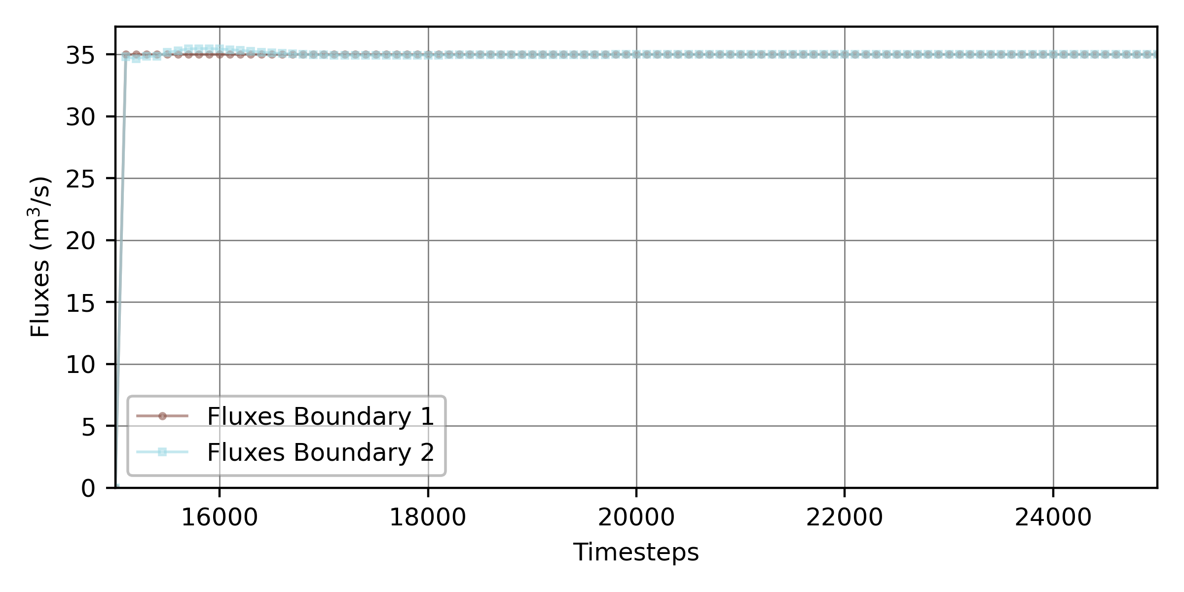
Figure 24:Flux convergence plot across the two boundaries of the hotstarted steady Telemac2d simulation, starting at a simulation time of 15000 timesteps.
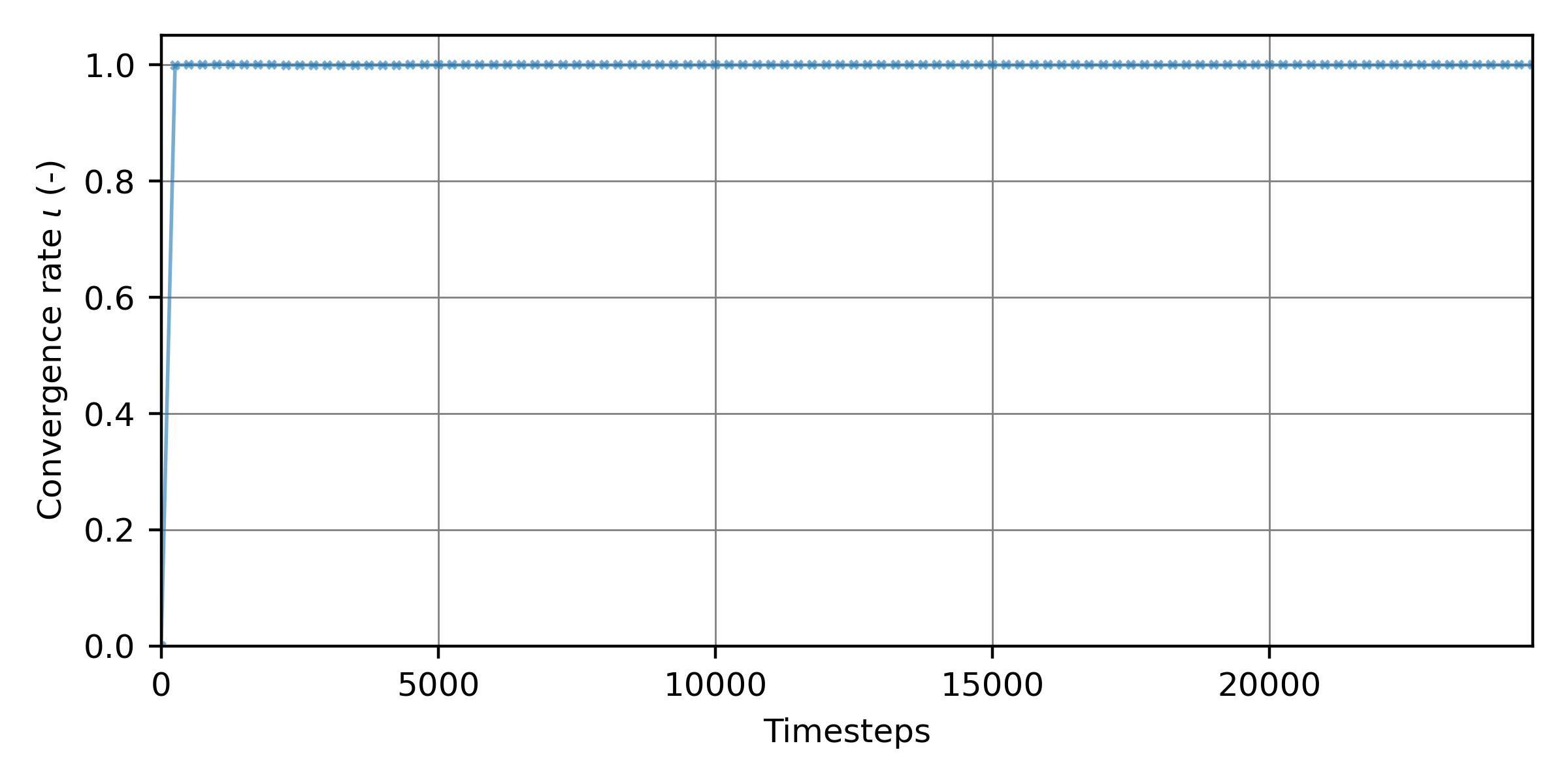
Figure 25:The convergence rate as a function 15000 simulation timesteps of the hotstarted steady 2d simulation with friction zones.
The required steady2d-zonal-ks.cas_2023-07-28-14h55min04s is available here for use with instructions from the spotlight chapter on convergence.
Working with Friction IDs
The friction zones can also be assigned through friction IDs, which then require setting up a zones file and friction data file, for example, as showcased in the Donau example (HOMETEL/examples/telemac2d/donau/).
In the showcase of this tutorial, working with friction tables required assigning the friction IDs defined in Tab. 1 to the BOTTOM FRICTION variable of the .slf mesh. The according files can be downloaded from our repositories:
get friction-with-IDs.xyz for interpolation in BlueKenue (see above, or directly
get qgismesh-frictionIDs.slf with
BOTTOMandFRIC_IDinstead ofBOTTOM FRICTIONStrickler roughness coefficients (uses default friction ID0).
friction.tbl & CAS
Create friction.tbl
Create a friction table file called friction.tbl (consider this friction.tbl template) with the following content, where the no entries (here starting in line 36) must correspond to the FRIC_ID assigned to the mesh (recall Fig. 20):
1 2 3 4 5 6 7 8 9 10 11 12 13 14 15 16 17 18 19 20 21 22 23 24 25 26 27 28 29 30 31 32 33 34 35 36 37 38 39 40 41* ----------------------------------------------------------------------------- * EXAMPLE ADAPTED FROM HOMETEL/examples/telemac2d/donau/ * * Implemented roughness laws: * NOFR : no friction (number of values) * HAAL : Haaland law (1 value : rB) * CHEZ : Chezy law (1 value : rB) * STRI : Strickler law (1 value : rB) * MANN : Manning law (1 value : rB) * NIKU : Nikuradse law (1 value : rB) * LOGW : Log Wall law (1 value : rB) * COWH : Colebrook-White law (2 values : rB, nDef) * * no : FRIC_ID assigned to the SLF mesh * * Riverbed * ------------- * typeB : roughness law for riverbed * rB : friction value for riverbed * nDefB : Mannings n for shallow flow zones * * Later walls (only with k-epsilon model) * ----------------------------------------- * typeS : roughness law for walls (option) * rS : friction value for walls (option) * nDefS : Mannings n for shallow waters (option) * * Non-submerged Vegetation (if needed) * ------------------------ * dp : mean diameter (option) * sp : averaged distance between roughness elements (option) * * ----------------------------------------------------------------------------- * no typeB rB NDefB typeS rS NDefS dp sp * 0 STRI 33.0 NULL 1 STRI 34.6 NULL 2 STRI 27.7 NULL 3 STRI 40.3 NULL 4 STRI 22.7 NULL END
Program 1:Example for a friction(.tbl) ID table.
Link friction.tbl in CAS file
To activate the friction data, add the following keywords to the .cas steering file, and deactivate any not-wall related FRICTION keywords:
/ steady2d-zonal-ks.cas steering file
/ ...
/ ACTIVATE these keywords
FRICTION DATA : YES / default is NO
FRICTION DATA FILE : 'friction.tbl'
MAXIMUM NUMBER OF FRICTION DOMAINS : 20 / consider to increase (default is 10)
/ steady2d-zonal-ks.cas steering file
/ ...
/ DEACTIVATE these keywords
/ LAW OF BOTTOM FRICTION : 3 / 3-Strickler
/ FRICTION COEFFICIENT : 80 / not use with zonal frictionSave the .cas steering file.
Run Telemac with Friction IDs
To run Telemac with friction IDs, make sure the above-indicated keywords are activated in the .cas steering file. The required files now embrace:
qgismesh
-frictionIDs .slf (mesh with FRIC_ID)boundaries.cli or hotstart conditions
r2dsteady-t15k.slf results file to enable the hotstart
steady2d
-zonal -ID .cas steering file updated keywords friction.tbl with friction IDs
With these files, activate and run Telemac as usual:
cd ~/telemac/v9.0.0/configs
source pysource.gfortranHPC.sh
cd ~/modeling/frictionID-tutorial/
telemac2d.py steady2d-zonal-ID.cas
Advanced Friction Routines
Modifying the FRICTION_USER Fortran subroutines is not mandatory for working with friction zones but can be useful for implementing or adapting the behavior of roughness laws. To activate a FRICTION_USER subroutine, for example, to implement the variable power equation from Ferguson (2007):
Copy the FICTION_USER subroutine template from
HOMETEL/sources/telemac2d/friction_user.finto a new folder of your simulation directory, for example:
/HOME/modeling/frictionID-tutorial/user_fortran/friction_user.fModify and save edits of
friction_user.f.Tell the steering (
.cas) file to use the modified FRICTION_USER Fortran file by adding the keywordFORTRAN FILE : 'user_fortran', which makes Telemac2d look up Fortran files in the/user_fortran/subfolder.
- Díaz Gómez, R., Pasternack, G. B., Guillon, H., Byrne, C. F., Schwindt, S., Larrieu, K. G., & Solis, S. S. (2022). Mapping Subaerial Sand-Gravel-Cobble Fluvial Sediment Facies Using Airborne Lidar and Machine Learning. Geomorphology, 401, 108106. https://www.sciencedirect.com/science/article/pii/S0169555X21005146
- Google. (nd). Google Satellite Imagery. https://mt1.google.com/vt/lyrs=s&x=%7Bx%7D&y=%7By%7D&z=%7Bz%7D
- Meyer-Peter, E., & Müller, R. (1948). Formulas for Bed-Load transport. IAHSR, Appendix 2, 2nd meeting, 39–65. http://resolver.tudelft.nl/uuid:4fda9b61-be28-4703-ab06-43cdc2a21bd7
- Strickler, A. (1923). Beiträge zur Frage der Geschwindigkeitsformel und der Rauhigkeitszahlen für Ströme, Kanäle und geschlossene Leitungen [Contributions to the question of the velocity formula and the roughness figures for streams, channels and closed pipes]. Mitteilungen Des Eidgenössischen Amtes Für Wasserwirtschaft, Switzerland, 16, 357.
- Rickenmann, D., & Recking, A. (2011). Evaluation of flow resistance in gravel-bed rivers through a large field data set. Water Resources Research, 47, W07538. 10.1029/2010WR009793
- Ferguson, R. (2007). Flow resistance equations for gravel- and boulder-bed streams. Water Resources Research, 43, W05427. 10.1029/2006WR005422