First Project
Once you installed QGIS, launch the program and walk through the following steps to make fundamental settings:
Open QGIS
Create a new project (New Empty Project)
Verify Project Properties:
In the top menu go to Project > Properties
Set the Coordinate Reference System CRS to EPSG:4326:
WGS84 (Coordinate Reference System) Bounds: -180.0000, -90.0000, 180.0000, 90.0000
Projected Bounds: -180.0000, -90.0000, 180.0000, 90.0000
Scope: Horizontal component of a 3d system. Used by the GPS satellite navigation system and for NATO military geodetic surveying.
Last Revised: Aug. 27, 2007
Area: World
Learn more at http://epsg.io
Retrieve point coordinates in any CRS format
Convert between different CRSs (e.g., convert 48.745, 9.103 from EPSG 3857 to EPSG 4326)
Save the project as qgis-project.qgz in a new qgis-exercise folder
Panels, Toolbars, and Plugins
Follow the below illustrated instructions to enable the QGIS Toolbox.
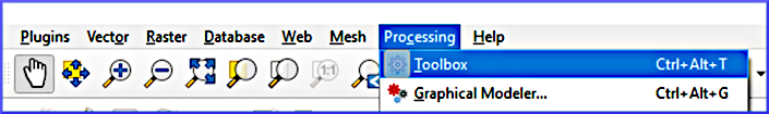
Figure 1:Open QGIS’ Toolbox window from the main menu.
In addition, the Digitizing Toolbar (View > Toolbars > check Digitizing Toolbar) is required to complete this tutorial.
The conversion between geospatial data types and numerical (computational) grids can be facilitated with plugins. To install any plugin in QGIS, go to the Plugins menu > Manage and Install Plugins... > All tab > Search... for a relevant plugin and install it.
In the context of river analysis, the following plugins are recommended and used at multiple places on this website:
BASEmesh is only one (very well working) mesh generator for QGIS and Tab. 1 lists of other plugins for generating computational meshes for numerical models along with target file formats and models
Basemaps for QGIS (Google or Open Street Maps Worldmap Tiles)
To add a base map (e.g., satellite data, streets, or administrative boundaries), go to the Browser, right-click on XYZ Tiles, select New Connection..., add a name, and a URL of an online base map. Once the new connection is added, it can be added to a QGIS project by drag and drop just like any other geodata layer. The below figure illustrates the procedure of adding a new connection and its XYZ tiles as a layer to the project. To overlay multiple basemaps (or any other layer), right-click on a layer, then Layer Properties > Transparency > modify the Opacity (e.g., to 50%).
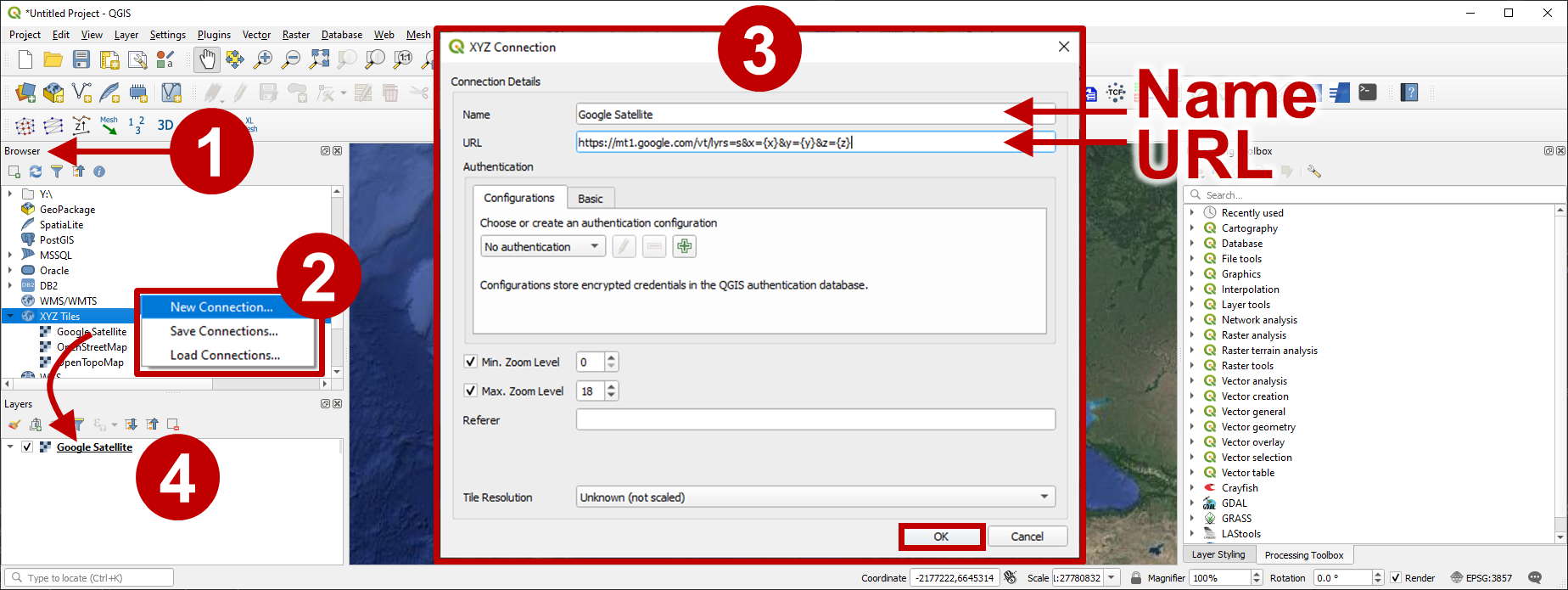
Add a base map to QGIS: (1) locate the Browser (2) right-click on XYZ-Tiles and select New Connection... (3) enter a Name and a URL (see below table) for the new connection, click OK (4) drag and drop the new tile (here: Google Satellite) into the Layers Panel.
Expand to watch the video tutorial on basemaps
Sebastian Schwindt@hydroinformatics on YouTube.
The following URL can be used for retrieving online XYZ tiles (more URLs can be found on the internet).
Create a Shapefile
This section guides through the creation of a point, a line, and a polygon Shapefile (vector data). To read more about such vector data and other spatially explicit data types, read the section on Geospatial Data.
Create a Point Shapefile
Start with loading satellite imagery and a street basemap (see above) in the layers pane. Zoom on central Europe and roughly locate Stuttgart in Southwest Germany. Find the heavily impaired Neckar River in the North of Stuttgart and move in the upstream direction (i.e., Eastern direction), pass the cities of Esslingen and Plochingen until you get to the confluence of the Neckar and the Fils rivers. From there, follow the Fils River in the upstream direction for a couple of hundred meters and locate the PEGELHAUS (i.e., a gauging station at the Fils River - click to visit). To facilitate finding the gauging station in the future, we will now create a point shapefile as explained in the following video and the analogous instructions below the video.
In the QGIS top menu go to Layer > Create Layer > New Shapefile Layer
Define a filename (e.g., gauges.shp - may not be longer than 13 characters), for instance, in a folder called qgis-exercise.
Geometry type:
MultiPointAdditional dimensions:
Z(+M Values)Add two new fields:
StnName(Text data)StnID(Whole number)
Edit/draw points
Toggle Editing (i.e., enable by clicking on the yellow pen
 ) > Digitizing Toolbar > Add Point Feature
Click on the PEGELHAUS to draw a point and set
StnName:PlochingenFilsStnID:00025
Add more points if you like.
Finalize the edits by clicking on Save Layer Edits
 > Stop (Toggle) Editing by clicking on the yellow pen symbol.
Improve the visualization by changing the symbology:
Double-click on the gauges layer > Symbology
Highlight Simple Marker, change to + symbol, and change fill color and size.
Highlight Marker and change the Opacity
Click Apply and OK
Verify the point settings in the Attribute Table (right-click on the gauges layer and select Attribute Table).
Create a Line Shapefile
Create a Line Shapefile called CenterLine.shp to draw a centerline of the Fils ± 200 m around the PEGELHAUS gauge, similar to the above-created point shapefile. Add one text field and call it RiverName. Then draw a line along the Fils River starting 200 m upstream and ending 200 m downstream of the PEGELHAUS by following the river on the OpenStreetMap layer. See more in the following video.
Create a Polygon Shapefile
To delineate different zones of roughness (e.g., as needed for a two-dimensional numerical model), create a Polygon Shapefile called FlowAreas.shp. The file will contain polygons zoning the considered section of the Fils into the floodplain and main channel bed. Name the first field AreaType (type: Text) and the second field ManningN (type: Decimal Number). See more in the following video and the instructions below the video.
To draw the polygons:
Enable snapping to avoid gaps between the floodplain and main channel polygons
Activate the snapping toolbar: View > Toolbars > Snapping Toolbar
Enable snapping from Snapping toolbar > Enable Snapping and Avoid Polygon Overlapping
To draw a polygon, go to the Digitizing Toolbar > Add Polygon Feature with the Digitize with Segment option enabled
Start drawing by clicking on the map (right-click finalizes Polygon)
Draw one polygon of the main channel and after finalizing set:
AreaType:MainChannelManningN:0.028
Draw two more polygons of the right-bank (RB) and left-bank (LB) floodplains, and set:
AreaType:FloodPlainRBandFloodPlainLBManningN:0.05(both)
If you made a drawing error, use either the Attribute Table to select and delete entire polygons, or use the vertex tool
 from the menu bar.
After drawing all polygons, Save edits and Toggle Editing (deactivate).
To improve the visualization, modify the Symbology to Categorized as a function of the
AreaTypefield: Keep Random Colors > Click on Classify > Apply and if you like the visualization, click OK.
Conversion: Rasterize (Polygon to Raster)
Many numerical models required that roughness is provided in Gridded Cell (Raster) Data format. To this end, this section features the conversion of the above-created polygon shapefile (FlowAreas.shp) to a roughness Gridded Cell (Raster) Data. The following video and the instructions below the video describe how the conversion works.
To convert a geospatial vector dataset, use the Rasterize tool:
In the QGIS menu bar make sure to enable the Processing Toolbox panel (View > Panels > Processing Toolbox)
In the Processing Toolbox > search (tap) Rasterize > select Rasterize (vector to raster)
In the Rasterize (Vector to Raster) window set:
Input layer:
FlowAreasField to use for a burn-in value:
ManningNOutput raster size units:
PixelsWidth/Horizontal resolution:
100(the smaller, the coarser the raster)Height/Vertical resolution:
100(the smaller, the coarser the raster)... scroll down ...
Output extent: click on the … button > Calculate from Layer >
FlowAreasRasterized (FILE NAME) > click on the … button > Save to File... >
roughness.tifClick Run
Set the Symbology to Singleband pseudocolor with Interpolation:
Discrete, Colorramp:Magma, Mode:Equal Interval> Apply. If the visualization is satisfactory, click OK.
Polygonize
The inverse operation of Rasterize is called Raster to Vector, which is documented at https://
Go to Raster (top menu) > Conversion > Polygonize (Raster to Vector)...
Input layer: select the raster to convert
Band number: the raster band for inferring the polygon value (i.e., field in the attribute table); some notes:
this algorithm will round decimals to integers (see video below)
alternatively, search Raster pixels to polygons in the Processing Toolbox, but it will create an excessive number of polygons
Name of the field to create: select a name for the polygon value field in the attribute table (no more than 10 characters)
Vectorized: define the directory and name for the new polygon shapefile
Click Run
To convert a Raster to a line/point (vector) shapfile, the options are the Contour tool (Raster menu > Extraction > Contour) or the Raster pixels to points algorithm (Processing toolbox > enter raster pixels to points). Also, have a look at the tutorials on geo file conversion with Python.
Working with Rasters
QGIS Raster Calculator (Map Algebra)
Some models preferably (default use) Manning’s n, others use the Strickler roughness coefficient , which is the inverse of Manning’s n (i.e., - read more about roughness coefficients in the 1d Hydraulics (Manning-Strickler Formula) exercise). Thus, transforming a Strickler roughness raster into a Manning roughness raster requires performing an algebraic raster (pixel-by-pixel) operation. The next video and the instructions below the video feature the usage of the QGIS Raster Calculator to perform such algebraic operations.
Start with opening Raster Calculator from QGIS menu bar (Raster > Raster Calculator...). Then, convert the above-created roughness.tif raster of Manning’s n values to a Strickler roughness raster:
Define an Output layer (e.g., qgis-exercise/roughness-stickler.tif) and keep the Output format of GeoTIFF.
Optionally select a layer extent corresponding to the above-created roughness.tif raster.
In the Raster Calculator Expression frame type 1, then click on the / button (Operators frame), then select roughness@1 from the Raster Bands frame.
The Raster Calculator Expression frame should now contain:
1 / "roughness@1", where the@sign refers to band number1.Click OK to run Raster Calculator.
After successful calculation, optionally modify the symbology of the new layer (roughness-stickler).
Raster to XYZ
Scientific data formats, such as HDF, work best with raw geospatial datasets like *.xyz files. A .*xyz file contains s only X, Y, and Z coordinates of points (i.e., point clouds) with or without a simple header. For instance, this eBook uses *.xyz data for the elevation interpolation of a computational mesh for the scientific numerical modeling software TELEMAC. To generate a *.xyz from a GeoTIFF raster use the following workflow:
In the Layers panel make sure to have raster layer imported for conversion and identify its No-Data value (Layer Properties > Information > Bands section > No-Data field show by default
-9999in QGIS).In QGIS top menu go to Raster > Conversion > Translate (Convert Format)...
In the Translate (Convert Format) window, make the following settings:
Input layer = the raster (e.g., a DEM) to convert
Advanced Parameters frame > Output data type > select Float32 (corresponds to single precision in numerical models)
Converted > ... button (at the end of the line) > Save to File... > define a File name such as
dem-pointsand selectXYZ files (*.xyz)in the Save as type field.Save and Run the translation (conversion).
The resulting *.xyz file contains also points with No-Data to fill void spaces in the rectangular image of the GeoTIFF (which QGIS did recognize as no-data pixels). The no-data points may make the *.xyz file unnecessarily heavy, in particular, when it is a DEM of a near-census natural river. To eliminate the unnecessary no data points, open the *.xyz file in spreadsheet software, such as Calc in LibreOffice and use the Sort tool (in Calc highlight all points go to Data > Sort...) to sort by Z values (largest to smallest) and then delete all rows that have the above-identified No-Data value (-9999) as Z value. Save the *.xyz file and close the spreadsheet software.
Shapefile to XYZ
Shapefiles do not have to be converted to GeoTIFF to create an *.xyz file. To create a *.xyz file from a shapefile:
Right click on the shapefile in the Layer panel > Export > Save Feature As....
Select Comma Separated Value (CSV) in the Format field.
Define a File name on clicking on the ... button.
In the Layer Options frame, select AS_XYZ in the GEOMETRY field and keep all other defaults.
Click OK to convert to CSV.
Open the CSV file in a text editor and use its find and replace function (usually
CTRL+ForCTRL+H) to replace all COMMA,by a space symbolSave the CSV file as
*.xyzfile.
To finalize the *.xyz file, open it in a text editor and add a header. For instance, use the following header to work with Blue Kenue:
:FileType xyz  ASCII  EnSim 1.0
:EndHeader
Save the changes. The *.xyz file is now slim and ready to use, for instance, for the TELEMAC pre-processing.
Create Layout and PDF / JPG (or other) Maps
Georeferenced images in GeoTIFF or other raster formats, possibly with super-positioned shapefiles on top, are handy and flexible for use with geospatial software, such as QGIS, but not appropriate for presentations or reports. For presentation purposes, geospatial imagery or maps should preferably be exported to common formats, such as the Portable Document Format (PDF) or JPEG/JPG. To create commonly formatted maps with QGIS, first, a new (print) layout needs to be created, which can then be exported to a common map format (e.g., along with a legend, a scale bar, and a North arrow). The following video and the descriptions below the video guide through the map creation process with QGIS.
Start with creating a new print layout by clicking on the Project drop-down menu, then select New Print Layout. In the new print layout prepare the map and export the map as follows:
Set a Layout title (e.g., exercise-layout).
In the new (exercise-layout) Layout:
Go to Add Item > Add Map.
Draw a rectangle that will contain the map.
Add Item > Add Scale Bar
To control scales and units shown in the scale bar:
In Items panel, highlight
<Scalebar>and find the Item Properties tab below.In the Item Properties tab modify units to your convenience.
Add Item > Add Legend
To control elements of the legend:
In Items panel, highlight
<Legend>and find the Item Properties tab below.In the Item Properties tab, find Legend Items > disable Auto update > remove OpenStreetMap and Google Satellite.
Toggle through other Items in the Add Item menu bar (e.g., Arrow for Northing).
Save the layout project (from top menu Layout > Save Project)
Export the map to common formats:
For JPG or PNG: Layout > Export as Image
For PDF: Layout > Export as PDF
Optional, for SVG-vector graphs: Layout > Export as SVG
QGIS has many other capacities, but this fundamental tutorial should have provided you with the necessary knowledge to leverage the power of QGIS for many applications.
PyQGIS: QGIS and Python
The QGIS graphical user interface (GUI) provides a Python command line (Plugins > Python Console), which enables to automate almost any mouse click in the GUI. This Python command line is referred to as PyQGIS and the QGIS developer docs provide instructions on how to import and run standalone Python scripts outside of the QGIS GUI. Here is the basic Python template to run a PyQGIS script:
from qgis.core import *

# define qgis installation location
QgsApplication.setPrefixPath("/path/to/qgis/installation", True)


# instantiate a QgsApplication, where the second argument (False) disables the GUI
qgs = QgsApplication([], False)


# load providers
qgs.initQgis()

# HERE GOES YOUR CUSTOM CODE

# exit the QGIS application to remove the provider and layer registries from memory
qgs.exitQgis()
However, when opening your system’s terminal or Anaconda Prompt to run a PyQGIS code, you may get stuck on the first line of code already: from qgis.core import * yields ImportError: No module named qgis.core. According to the QGIS developer docs, this error happens because your system’s Python does not know where the PyQGIS environment lives. To make your terminal recognize PyQGIS, take the following action according to your system:
Open Terminal and install python-qgis:
sudo apt install python-qgisAfter the successful installation, try if you can now import qgis.core:
USER@computer:~$ python
Python 3.8.10 (default, Nov 14 2022, 12:59:47)
[GCC 9.4.0] on linux
Type "help", "copyright", "credits" or "license" for more information.
>>> from qgis.core import *
>>> exit()
If from qgis.core import * did not throw any error, you are all set and can stop reading. Otherwise, find and open your .bashrc file (Debian/Ubuntu/Mint: /home/USERNAME/.bashrc). Note that files starting with a . name are hidden on Linux and become visible by toggling with simultaneously pressing the CTRL+H keys.
At the bottom of .bashrc add the following
export PYTHONPATH=/<qgispath>/share/qgis/pythonThe <qgispath> expression should be replaced by the location where the PyQGIS environment lives. To find out where that is, tap (in Terminal):
dpkg-query -L python-qgisThis points to where PyQGIS lives, which, on Ubuntu/Mint typically is:
/usr/lib/python3/dist-packages/Thus, in this case add to .bashrc:
export PYTHONPATH=/usr/lib/python3/dist-packages/Afterward, log out and re-login to your system (i.e., reload .bashrc). The command from qgis.core import * should now work in Python.
Make sure your system knows the where PyGIS lives by adding the following line to the Environment Variables (Windows 10: My Computer > Properties > Advanced System Settings > Environment Variables). Replace <qgispath> with the path where QGIS lives on your system.
Variable name =
PYTHONPATHVariable value =
C:\<qgispath>\python
Or use the Windows prompt:
set PYTHONPATH=C:\<qgispath>\python- Shewchuk, J. R. (1996). Triangle: Engineering a 2D quality mesh generator and Delaunay triangulator. In M. C. Lin & D. Manocha (Eds.), Applied Computational Geometry Towards Geometric Engineering (pp. 203–222). Springer. 10.1007/BFb0014497