In addition to the SMS 2dm file from the Pre-processing with QGIS tutorial, the numerical engine of BASEMENT needs a model setup file (model.json) and a simulation file (simulation.json), which both are created automatically by BASEMENT.
The following sections describe how to make BASEMENT creating the required JSON files in a project directory such as C:\Basement\steady2d-tutorial\ (Windows) or ~/Basement/steady2d-tutorial/ (Linux). Therefore, the first step is to create a project directory (folder).
Place the following input files in the project folder:
The SMS 2dm file with interpolated bottom elevations from the Pre-processing with QGIS tutorial (prepro-tutorial_quality-mesh-interp.2dm).
A steady discharge inflow file (flat hydrograph) for the upstream boundary condition can be downloaded here (if necessary copy the file contents locally into a text editor and save the file as steady-inflow.txt in the project directory).
Initiate the Model
This section guides through the model setup, which is saved in a file called model.json (here: in the folder /steady2d-tutorial/). Start BASEMENT and select the folder created above as the Scenario Directory (see Fig. 1).
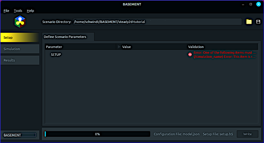
Figure 1:BASEMENT’s welcome screen after selecting a Scenario Directory with the Save Project button in the top-right corner. The directory references may look different on other platforms (e.g., start with "C:/... on Windows).
Next, left-click on SETUP, then right-click and select Add item BASEHPC. A new tab called Define Scenario Parameters opens. For the moment, ignore the warning and error messages (red tags) and define a simulation_name:
Right-click on SETUP and select Add item ‘simulation_name’. A new entry called simulation_name will appear at the bottom of the Define Scenario Parameters tab.
Scroll to the bottom, double-click on “RUNFILE” (default value behind simulation_name) and replace
RUNFILEwithsteady2d.
Scroll back to the top, and save the project, to proceed with the next sections.
Geometry and Regions
The GEOMETRY group in the Define Scenario Parameters tab tells the model, which SMS 2dm mesh file to use and enables the definition of region and liquid boundary properties. To this end, make the following settings:
Double-click on the Value field of the mesh_file row and click on the folder symbol

In the popup window select the previously created prepro-tutorial_quality-mesh-interp.2dm and hit Enter.
The mesh created in the last chapter contains multiple regions, which also need to be defined in the model setup:
Right-click on GEOMETRY > Add item REGIONDEF
Add 5 region items by right-clicking on the new REGIONDEF entry > Add item. The number of regions should correspond to the regions defined in the pre-processing tutorial, which are also below-listed in Tab. 1.
Define the five regions by a right-click on index > Add item.
Every index [0] item gets an integer number assigned corresponding to the MATID field in the region points shapefile (see the Region Markers section in the Pre-processing with QGIS tutorial).
The name of every region item corresponds to the type field of the MATID.
Table 1 summarizes the required region definitions. With the regions and the mesh file defined, the GEOMETRY group should resemble Fig. 2.
Table 1:REGIONDEF items and their definitions to be defined in BASEMENT’s model setup.
REGIONDEF | [0] | [1] | [2] | [3] | [4] |
|---|---|---|---|---|---|
index [0] | 1 | 2 | 3 | 4 | 5 |
name | riverbed | block_ramp | gravel_bank | floodplain | sand_deposit |
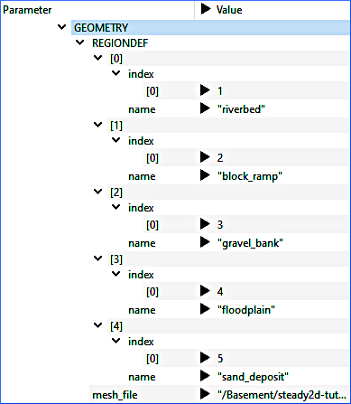
Figure 2:The GEOMETRY group with REGIONDEFs and the reference to the height-interpolated mesh file (prepro-tutorial_quality-mesh-interp.2dm).
The liquid (hydraulic) boundaries from the pre-processing tutorial geographically define inflow and outflow lines with stringdef attributes that are incorporated in the mesh file (prepro-tutorial_quality-mesh-interp.2dm) with height (elevation) information. To communicate BASEMENT the types and the properties of the liquid boundaries, complete the GEOMETRY section:
Right-click on GEOMETRY > Add item STRINGDEF.
Right-click on the new STRINGDEF item and select Add item two times. Thus, two items should be available to define the upstream and downstream liquid boundaries.
Define STRINGDEF item [0] with:
name =
inflowupstream_direction =
right
Define STRINGDEF item [1] with:
name =
outflowupstream_direction =
right
If you used the provided liquid boundaries shapefile to create the mesh file, the upstream_direction must be right. Figure 3 shows the definition of the STRINGDEF items using the provided liquid boundaries shapefile.
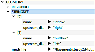
Figure 3:The GEOMETRY group with STRINGDEFs using the provided liquid boundaries shapefile in the computational mesh.
Hydraulics
Hydraulic model characteristics that apply to the above-defined geometry setup are defined in the HYDRAULICS group of BASEMENT’s model setup. This tutorial uses the default for INITIAL conditions, which is “dry”. Also keep the default PARAMETERS for CFL = 0.9, fluid_density = 1000.0, max_time_step = 100.0, and minimum_water_depth = 0.01.
Hydraulic quantities, such as water depth and discharge, must be assigned to the liquid boundaries defined above so that the numerical model knows how much water it must make running through the model. Therefore, add the following boundary definitions in the HYDRAULICS group:
Right-click on HYDRAULICS and select Add item BOUNDARY.
Right-click on the new BOUNDARY item and select Add item STANDARD.
Right-click two times on the new STANDARD item and select Add item each time. Thus, there should be two items [0] and [1] to define the inflow and outflow conditions, respectively.
Define item [0] with the following inflow conditions:
For name enter
inflow.For string_name select inflow (defined above).
For type select
uniform_inRight-click on [0] and select Add item ‘slope’.
For the new slope item, define a value of
0.0044. After entering the slope value, check if BASEMENT correctly understood the decimal separator: make sure to use the decimal separator of your system locale (e.g., on a European keyboard, it may be necessary to use,instead of.).Right-click on [0] and select Add item ‘discharge_file’.
In the new discharge_file row, click on the folder symbol to select the above-described steady-inflow.txt file.
Define item [1] with the following outflow conditions:
For name tap
outflow.For string_name select the above-defined
outflowSTRINGDEF.For type select
uniform_outRight-click on [1] and select Add item ‘slope’.
For the new slope item, define a value of
0.0044.
Figure 4 shows the definitions of STANDARD BOUNDARY items in BASEMENT’s HYDRAULIC model setup group.
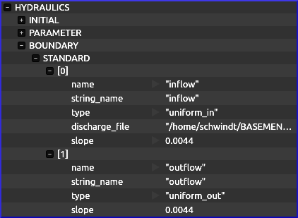
Figure 4:The HYDRAULIC entry with BOUNDARY > STANDARD definitions for the upstream (inflow) and downstream (outflow) liquid model boundaries.
Every surface has imperfections that cause turbulence when fluids such as water flow over it. The turbulences caused by surface imperfections result in decelerated flows near the surface. Since the water in rivers is almost always very close to the Earth’s surface in the form of the riverbed relative to the imperfections of a riverbed, the influence of friction-induced turbulence is considerable. In hydrodynamic models, the friction-induced turbulence of the rough surface of riverbeds is accounted for by a friction coefficient, such as the Strickler coefficient or its inverse value called Manning’s . The exercise on 1d Hydraulics (Manning-Strickler Formula) in the Python chapter explains both roughness coefficients in more detail. This tutorial uses a global Strickler coefficient of =30 (fictive units of m/s), which accounts for the characteristics of a meandering gravel-cobble riverbed Strickler, 1923. To this end, right-click on the HYDRAULICS group and select Add item FRICTION. Define the new FRICTION item with:
default_friction = 30.0
type =
strickler
Next, assign region-specific Strickler values for the five regions defined in Tab. 1:
Right-click on FRICTION > Add item regions.
Right-click on the new regions item and select Add item (five times for the five regions).
Assign the friction and region_name values listed in Tab. 2 to the five regions items.
Table 2:Strickler values for HYDRAULIC FRICTION regions.
Region | Riverbed | Block ramps | Gravel banks | Floodplains | Sand |
|---|---|---|---|---|---|
friction | 34 | 18 | 24 | 14 | 39 |
region_name | riverbed | block_ramp | gravel_bank | floodplain | sand_deposit |
Figure 5 shows the definition of the hydraulic FRICTION items in BASEMENT’s model setup.
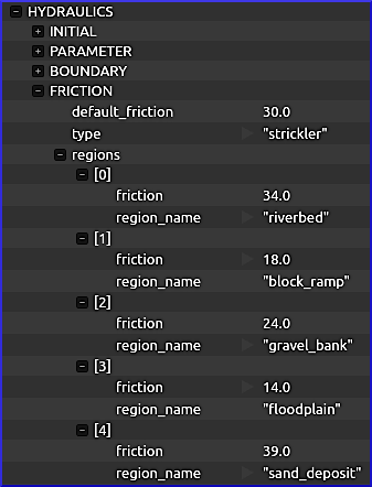
Figure 5:The HYDRAULICS group with FRICTION definitions for the model and its regions.
Physical Properties
The definition of the PHYSICAL_PROPERTIES group is mandatory for BASEPLANE_2D. This tutorial uses the default physical properties (i.e., gravity is 9.81).
Write Setup File
Make sure that any potential warning or error message is resolved and that the model setup resembles Fig. 6. Before exporting the project, save the simulation setup (click on the disk symbol in the top-right corner in Fig. 6). Double-check that BASEMENT correctly wrote the files model.json, simulation.json, and results.json in the project directory (e.g., /Basement/steady2d-tutorial/). Export the model setup by clicking on the Write button (bottom-right corner in Fig. 6).
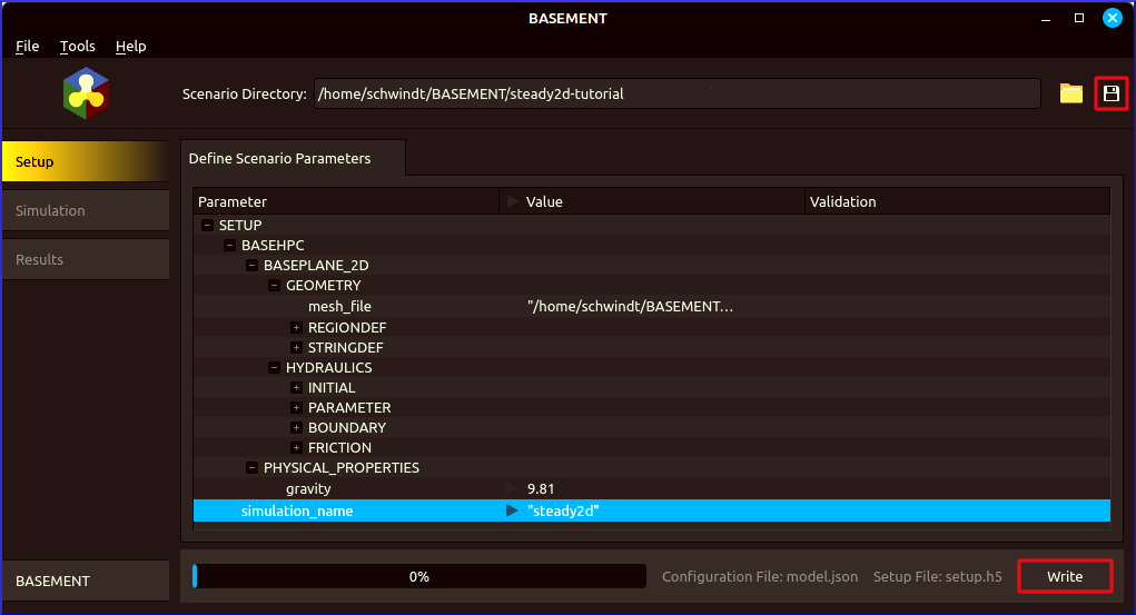
Figure 6:The final model setup to export (write) to a setup (*.h5 HDF) file.
The Console tab automatically activates and informs about the export progress. If the Error Output canvas is not empty, check the error messages and troubleshoot the causes.
Setup Simulation File
After the successful export of the model setup, the Simulation ribbon (on the left in Fig. 6) becomes available for setting up the simulation.json file in the project folder. Click on the Simulation ribbon to setup the simulation.json file:
Right-click on the SIMULATION group in the activated Define Simulation Run tab and select Add item ‘OUTPUT’.
Right-click on the new OUTPUT item to define five output types:
[0] =
water_depth[1] =
water_surface[2] =
bottom_elevation[3] =
flow_velocity[4] =
ns_hyd_discharge
Right-click on the SIMULATION group and select Add item ‘TIME’.
Define the TIME item with:
end =
15000.0out =
1000.0start =
0.0
The values defined in the TIME section refer to the same time units as defined in the above-downloaded and linked steady-inflow.txt file. Figure 7 shows BASEMENT with the definitions in the Simulation ribbon.
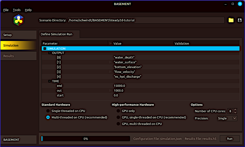
Figure 7:The setup of the Simulation ribbon with the definition of five output parameters and the simulation time.
Run Simulation (Steady 2d)
The simulation can be run with different options that mainly affect the computing time (bottom of Fig. 7).
The Standard Hardware frame enables to switch between single and multi-threaded CPU usage. The default option is multi-threaded, which is strongly recommended with contemporary computers.
The High-performance Hardware frame enables to use a graphical processing unit (GPU), which can be significantly faster than CPU, but only when a powerful graphics processor is available. A standard-slow GPU will not have an advantage and may even slow down the computation. If you are not sure about the GPU of your computer, keep the default options (all void).
The Options frame enables to choose:
The Number of CPU cores, which enables to use multiple CPUs of a computer. Contemporary computers mostly have at least 8 cores that can all be used when you are working on a server or computer that has no other purpose than running numerical models. Otherwise, keep the system functional while the simulation is running by using half the number of available cores.
Numeric precision; for faster simulations, select Single precision. For this tutorial, Double precision will work sufficiently fast as well, but in practice, Single precision is mostly sufficient and considerably faster.
To start the simulation click on the Run button on the bottom-right of the BASEMENT window. Depending on the hardware and performance settings (e.g., number of CPUs), the simulation of the tutorial model takes approximately 1-10 minutes. BASEMENT informs about the simulation progress in the Console Output frame, where the Error Output frame should remain empty (see Fig. 8). If any error occurs, go back to the above sections (or even to the mesh generation tutorial) to fix errors.
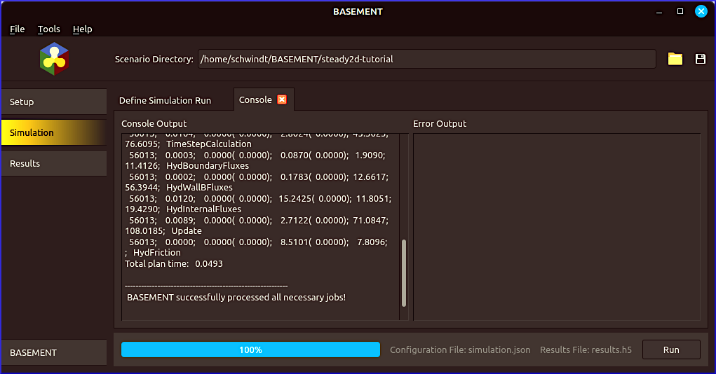
Figure 8:BASEMENT after successful simulation.
Export Simulation Results
Once the simulation successfully finished, go to BASEMENT’s Results ribbon. Find the RESULTS group in the Export Simulation Results tab and:
Right-click on the RESULTS group and select Add item ‘EXPORT’.
Right-click on the new EXPORT item and select Add item.
Select xdmf in the format field of the new item [0].
Save the project (disk symbol in the top-right corner) and find the Export indicated in Fig. 9). The export of the simulation outputs to results.xdmf will be confirmed in the Console Output frame.
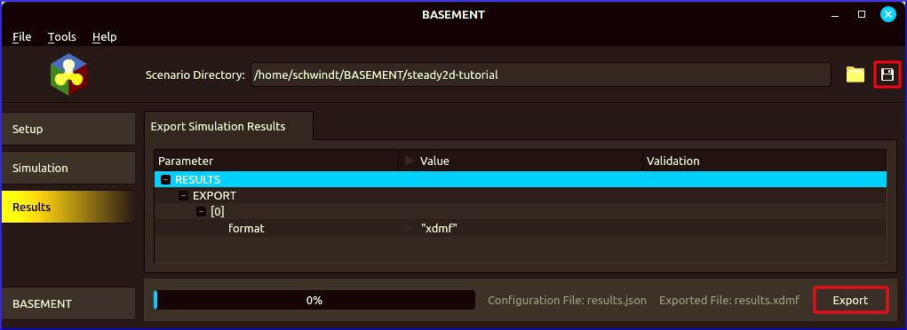
Figure 9:Setup of the Results ribbon after a successful simulation.
Post-processing with QGIS
Start QGIS and create a new project or re-use the project from the Pre-processing with QGIS tutorial. Save the new project with (a different) meaningful filename in the BASEMENT modeling folder (e.g., /Basement/steady2d/postpro-tutorial.qgz). Setup the project similarly as in the pre-processing:
Use the coordinate reference system Germany_Zone_4 (QGIS Setup section).
Add a satellite imagery basemap (XYZ tile) to facilitate the interpretation of the simulation results.
Import the height-interpolated quality mesh prepro-tutorial_quality-mesh-interp.2dm (Layer > Add Layer > Add Mesh Layer...).
Import results.xdmf
The simulation results file results.xdmf can be loaded in QGIS as an additional data source of the height-interpolated quality mesh (prepro-tutorial_quality-mesh-interp.2dm) from the pre-processing tutorial:
In the Layers panel, double-click on prepro-tutorial_quality-mesh-interp.2dm to open the Layer Properties window.
In the Layer Properties window, go to the Source ribbon.
In the Available Datasets frame (see Fig. 10) click on the Assign Extra Data Set to Mesh button
 and choose
 results.xdmf.
In the Static Dataset frame, select a Scalar Dataset Group and use the maximum timestep (i.e.,
625 d 00:00:00in the case of simulation time =15000 with an output interval of 1000).Click on Apply and OK.
Figure 10 shows an exemplary setup of the output data interpolation on the computational mesh. To visualize other output parameters and/or other simulation timesteps, vary the definitions in the Static Dataset frame.
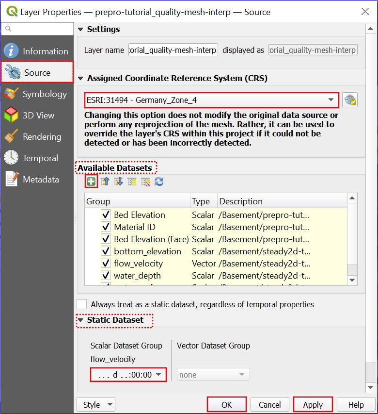
Figure 10:Assign mesh data to the computational mesh.
To improve the visualization of the results, re-open the Layer Properties of the mesh layer and go to the Symbology ribbon. Visualize a simulation output parameter, such as flow_velocity, as follows:
In the Settings tab (hammer symbol in the top-left corner highlighted in Fig. 11) find the Groups listbox.
In the Groups listbox, find the parameter to visualize (e.g., flow_velocity) and enable the contours symbol.
Switch to the Contours tab next to the Settings tab (highlighted box in the top-left of Fig. 11) and select a Color Ramp.
After defining a visualization click Apply and OK.
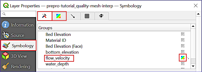
Figure 11:Visualize the flow_velocity parameter with the Symbology controls. The red boxes highlight relevant tabs and entries.
Figure 12 illustrates a visualization of the flow velocity at the end of the simulation. The flow velocity results are also available as a video sequence (download).
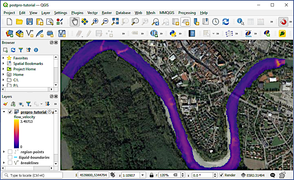
Figure 12:After application of the above Symbology settings: The flow velocity is illustrated in red shades.
Rasterize Outputs
The Gridded Cell (Raster) Data format is useful for many post-processing tasks such as map algebra (e.g., for habitat analysis or the assessment of inundation area and depth). To this end, QGIS provides the Rasterize mesh dataset tool for converting mesh data at any simulation timestep to a Raster (e.g., as GeoTIFF). To open the Rasterize mesh dataset tool, go to either Processing > Toolbox or make sure that the View > Panels > Processing Toolbox is checked. In the Processing Toolbox click on the Mesh group and double click on Rasterize mesh dataset (see also Fig. 13).
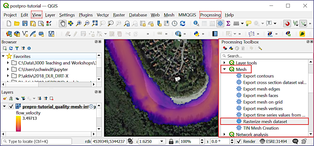
Figure 13:Open the Rasterize mesh tool in QGIS’ Processing Toolbox.
Make the following settings in the Rasterize window (see also Fig. 14):
Set the Input Mesh Layer to
prepro-tutorial_quality-mesh-interp.In the Dataset groups frame, click on the ... button > Select in Available Dataset Groups and select one parameter (e.g., flow_velocity). Then, clicking on the Go back
 button. Make sure that the Dataset groups canvas contains only 1 selected option. Otherwise, the tool will create a messy multiband Raster.
In the Dataset time frame, check the Dataset group time step radio button and select the last simulation timestep (i.e.,
625 d 00:00:00).In the Extent [optional] field, click on the ... button > Calculate from Layer > prepro-tutorial_quality-mesh-interp.
For Pixel size tap
2.0meters (the larger this number, the coarser will be the output raster).For Output coordinate system select
Project CRS: ESRI:31494 - Germany_Zone_4.Define an Output raster layer by clicking on the ... button > Save to File. Go to the target directory (e.g.,
C:/Basement/steady2-tutorial/) and enter a raster name, such asu-end.tif(ufor flow velocity,endfor last timestep, and.tiffor GeoTIFF). Click Save.Click on the Run button to start rasterizing the mesh dataset.
After the successful rasterization, close the Rasterize Mesh Dataset window with a click on the Close button.
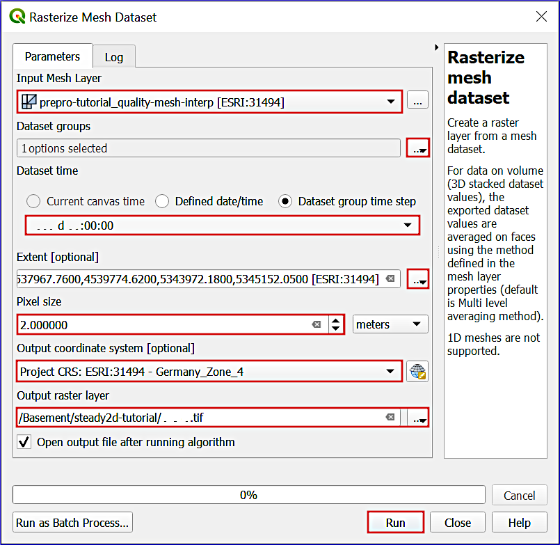
Figure 14:Settings to export simulation results with QGIS’s Rasterize tool.
To enhance the visualization of the new (flow velocity) raster, double-click on the new raster in the Layers panel and switch to the Symbology tab. Select Singleband pseudocolor for Render type (in the top region of the window) and a Color ramp. To suppress zero-value pixels, double-click on the Color of the 0-Value field, and in the Select color window reduce the Opacity to 0. Figure 15 shows an example visualization of the exported flow velocity raster.
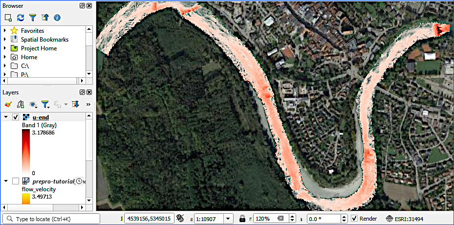
Figure 15:A Singleband pseudocolor (Layer Properties > Symbology) represents the exported GeoTIFF flow velocity raster with a Reds color ramp and zero-value pixels set to zero-opacity, superpositioned on google satellite imagery Google, n.d..
Mesh Visualization with Crayfish
The open-source Crayfish plugin enables the visualization of mesh values (e.g., change of node values over time) with many features, such as exporting video animations of model results. To create a video of, for instance, the flow velocity outputs at the 1+15 simulation timesteps, use the Crayfish plugin as follows:
In QGIS, make sure the Crayfish plugin is installed (recall the QGIS instructions).
In the Layer panel, select prepro-tutorial_quality-mesh-interp.
With prepro-tutorial_quality-mesh-interp selected, go to Mesh (top dropdown menu) > Crayfish > Export Animation ... (if the layer is not highlighted, an error message pops up: Please select a Mesh Layer for export).
In the Export Animation window, go to the General tab and define an output file name by clicking on the ... button (e.g.,
velocity-video.avi).Click OK.
The first time that a video is exported, Crayfish will require the definition of an FFmpeg video encoder and guide through the installation (if required). Follow the instructions and re-start exporting the video.
Post-processing with ParaView
ParaView is freely available visualization software, which enables plotting and processing BASEMENT’s results.xdmf file for scientific purposes. Download and install (requires Admin/sudo rights) the latest version of ParaView from their website (if not yet done).
Import results.xdmf
Open ParaView and click on the folder icon (top-left of the window indicated in Fig. 16) to load the simulation results file (results.xdmf). ParaView might ask to choose an appropriate XDMF read plugin: Select XDMF Reader and click OK. Now, the results.xdmf should be visible in the Pipeline Browser and the Apply button has turned green (click on it).
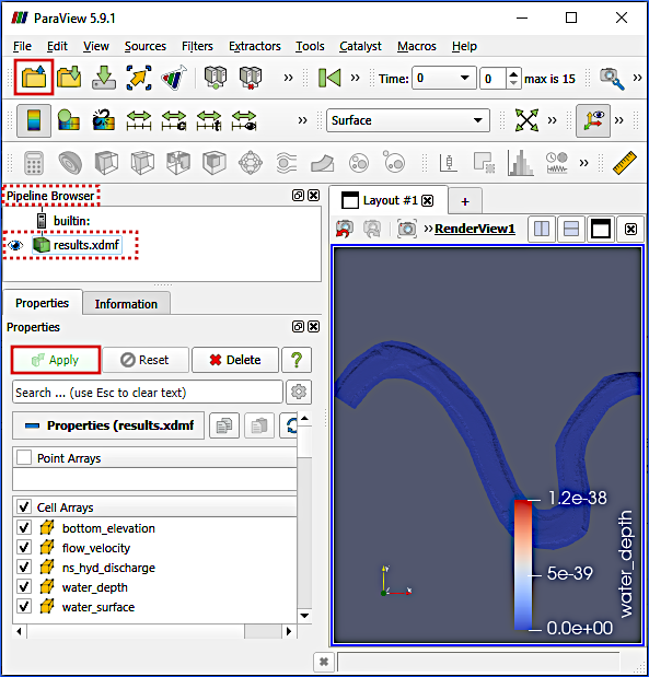
Figure 16:ParaView after successful import of the model results (results.xdmf).
Visualize Parameters
ParaView shows by default one of the result parameters at timestep 0 (i.e., bare, dry terrain). To explore other parameters, select them in the dropdown menu of the Active Variable Controls menu bar (red highlight box in Fig. 17). The Active Variable Controls menu bar also contains options for manipulating the color range and legend. Toggle through the timesteps by using the video control buttons in the VCR Controls toolbar (light blue highlight box in Fig. 17).
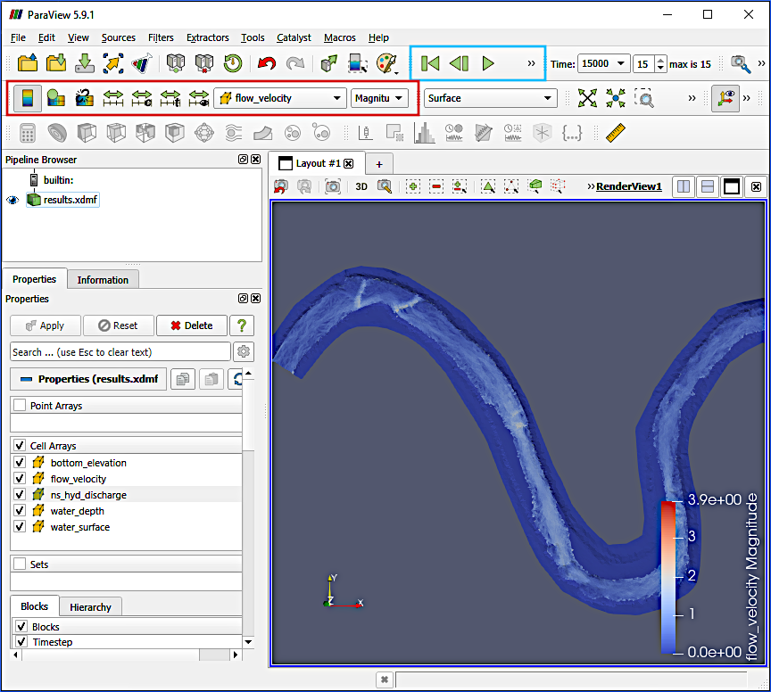
Figure 17:The Active Variable Controls (red box) and VCR Controls (light blue box) in ParaView to visualize output parameters at different timesteps.
To export an animation of an output parameter over time as movie (e.g., avi) or image (e.g., jpg, png, tiff) go to File > Save Animation....
Save Project Pipeline
With its approach of sequences of programmable filter application, ParaView saves a Current State in the PVSM format rather than a project as in QGIS. The current state of a dataset in ParaView can be saved as pvsm file via File > Save State File. Save the current state of the tutorial ParaView project, for instance, in the simulation folder as pv-project.pvsm. To load an existing ParaView state (i.e., project), go to File > Load state.
Export Data
Similar to QGIS, output parameter datasets can be extracted, manipulated, or transformed in ParaView. For this purpose, programmable filters can be applied to the original dataset in ParaView to calculate (i.e., apply the Calculator  filter), for example, the Froude number from the water depth and flow velocity datasets (read more in the ParaView Wiki). This tutorial only features the export of mesh point data to a CSV file with programmable filters:
Make sure that the Time in the Current Time Controls toolbar (light blue box in Fig. 18) is set to 15000 (maximum timestep).
In the Pipeline Browser, right-click on
results.xdmf> Add Filter > Alphabetical (i.e., a list of all available filters) > Cell Centers.In the CellCenters1 Properties, check the Vertex Cells box and click on the now again green Apply button (see Fig. 18).
To save the currently active vertex data press
CTRL+Son the keyboard, which opens a Save File dialogue window. In the Save File window:Navigate to a target folder (e.g., the simulation folder
/Basement/steady2d-tutorial/)Enter a File name (e.g.,
flow_velocity.csv)In the Files of type drop-down field, select Comma or Tab Delimited Files(
*.csv *.tsv *.txt).Click OK.
The Configure Writer (CSV Writer) window opens:
Check the Choose Array To Write box.
Select flow_velocity points only (or more/other parameters).
Keep all other defaults.
Click OK.
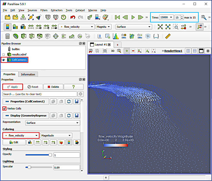
Figure 18:Application of the CellCenters programmable filter in ParaView, with the maximum timestep defined in the Current Time Controls toolbar (light blue box).
Now, a flow_velocity.CSV file has been written that contains point coordinates (x, y, and z coordinates) and flow_velocity in x (flow_velocity:0) and y (flow_velocity:1) directions. The flow_velocity:2 (z-direction) is always zero in this 2d simulation. The flow_velocity.CSV file can also be used with QGIS (for instance, in QGIS go to Layer > Add Layer > Add Delimited Text Layer... > select flow_velocity.csv, assign the correct columns and separators > click Add).
Python Simulation Verification
BASEMENT’s developers at the ETH Zurich provide a suite of Python scripts for post-processing the simulation results. For the here used BASEMENT v3, download the Python script BMv3NodestringResults
To run the Python script, install Python for your platform along with the numpy and h5py packages.
For running the Python script on any platform:
Optionally activate the relevant Python (conda or venv) environment.
cd(change directory) into the simulation folder.Run
python BMv3NodestringResults.py.
In detail, this looks as follows:
Launch Windows or Anaconda Prompt and tap (requires that the conda environment flussenv is installed):
conda activate flussenv
cd C:\Basement\steady2d-tutorial\
python BMv3NodestringResults.py
Launch Linux Terminal and tap (requires that the pip environment vflussenv is installed in the HOME directory):
cd ~
source vflussenv/bin/activate
cd /Basement/steady2d-tutorial/
python BMv3NodestringResults.py
If vflussenv is installed in another directory than HOME, replace cd ~ in the first line of the above code block with the parent installation directory of vflussenv.
Figure 19 illustrates running BMv3NodestringResults.py on Windows in Anaconda Prompt.
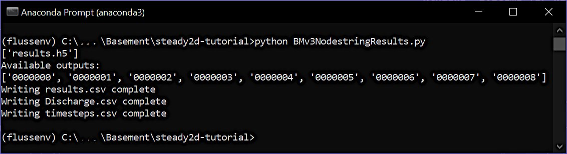
Figure 19:A Python Anaconda Prompt window running BMv3NodestringResults.py
Running the Python script generates three CSV files that contain values at the user-defined STRINGDEFs:
Discharge.csv contains inflow and outflow discharges.
results.csv contains any OUTPUT parameter defined in the simulation setup file.
timestep.csv lists the number of OUTPUT parameter timesteps.
The primarily important file is Discharge.csv, from which can be read when inflow and outflow converge in a steady-state simulation (i.e., the simulation stabilizes). A steady simulation in which the sum of all inflows does not equal all outflows must be considered erroneous. For instance, if the sum of outflows in the last timestep is smaller than the sum of inflows, then the simulation time is too short. The diagram in Fig. 20 plots inflow and outflow for the simulation setup of this tutorial. The diagram suggests that the model reaches stability after timestep 11 (simulation time ). Thus, the simulation time could be limited to , but a simulation time of would be too short.
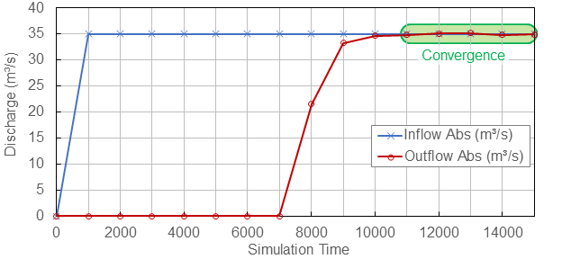
Figure 20:Convergence of inflow and outflow at the model boundaries.
- What next?
- The verification of the model stability represents only one step on the pathway to a useable model in practice. Before a numerical model can be used for simulating decision-making scenarios, it must be calibrated and validated with measurement data (similar to TELEMAC hydrodynamics).
- Strickler, A. (1923). Beiträge zur Frage der Geschwindigkeitsformel und der Rauhigkeitszahlen für Ströme, Kanäle und geschlossene Leitungen [Contributions to the question of the velocity formula and the roughness figures for streams, channels and closed pipes]. Mitteilungen Des Eidgenössischen Amtes Für Wasserwirtschaft, Switzerland, 16, 357.
- Google. (nd). Google Satellite Imagery. https://mt1.google.com/vt/lyrs=s&x=%7Bx%7D&y=%7By%7D&z=%7Bz%7D