Convergence (Quantitative) - Hydro-Informatics

Requirements

Complete the Telemac steady 2d tutorial (or similar).
The MASS-BALANCE : YES and/or PRINTING CUMULATED FLOWRATES : YES keywords must have been used in the steering (.cas) file to print mass fluxes across liquid boundaries in the Terminal.
The Telemac simulation must have been running with the s flag (more details below):

telemac2d.py [STUDY-NAME].cas -s

An installation of Python along with the numpy, pandas, and matplotlib libraries (see the Python installation guide), even though flusstools is not required).

All required simulation files for this tutorial can be downloaded from the hydro-informatics/telemac repository on GitHub (see details below).

This chapter uses the simulation files from the Telemac steady 2d tutorial, but with a slightly different definition of timesteps and printout periods:

/ steady2d-conv.cas
TIME STEP : 1.
NUMBER OF TIME STEPS : 10000
GRAPHIC PRINTOUT PERIOD : 50
LISTING PRINTOUT PERIOD : 50

Additionally, the simulation was rerun with the -s flag, which saves the simulation state in a file called similar to [FILE-NAME].cas_YEAR-MM-DD-HHhMMminSSs.sortie.

telemac2d.py steady2d-conv.cas -s

Both the steering .cas and .sortie files can be downloaded from the hydro-informatics.com repositories:

Extract and Check Flux Data¶

The Telemac jupyter notebook templates (HOMETEL/notebooks/ > data_manip/extraction/*.ipynb or workshops/exo_fluxes.ipynb) provide some guidance for extracting data from simulation results, which can be tweaked into a generally applicable framework for observing mass convergence at the boundaries as a function of the defined NUMBER OF TIME STEPS. However, the notebook templates do not work straightforwardly, which is why the following paragraphs describe a simple, minimalist Python tweak called pythomac, developed by hydro-informatics.com. There are three options for working with our codes, and all of them require having an installation of Python along with the numpy, pandas, and matplotlib libraries (see the Python installation guide):

pip-install pythomac

clone pythomac

download pythomac as zip

Pip-install the pythomac package:

pip install pythomac

Clone the pythomac repository from GitHub:

git clone https://github.com/hydro-informatics/pythomac.git

Copy-paste the folder pythomac/pythomac/ into your simulation directory. That is, make sure that the Python script /HOME/pythomac/extract_fluxes.py (among others) is correctly located, next to /HOME/your-simulation-dir/steady2d.cas.

Expand to see the code in the extract_fluxes.py Python script:

""" Extract data from a Telemac simulation that has already been running.
The codes are inspired by the following jupyter notebook:
    HOMETEL/notebooks/data_manip/extraction/output_file_extraction.ipynb
 which uses the following example case:
    /examples/telemac2d/bump/t2d_bump_FE.cas
"""

# retrieve file paths - this script must be stored in the directory where the simulation lives
import sys
import os
# data processing
import pandas as pd
import numpy as np
# plotting
import matplotlib
import matplotlib.pyplot as plt

sys.path.insert(0, os.path.dirname(os.path.realpath(__file__)))
# Telemac stuff
from parser_output import get_latest_output_files
from parser_output import OutputFileData


def extract_fluxes(
        model_directory="",
        cas_name="steady2d.cas",
        plotting=True
):
    """This function writes a .csv file and an x-y plot of fluxes across the boundaries of a Telemac2d model. It auto-
        matically place the .csv and .png plot files into the simulation directory (i.e., where the .cas file is).

    Notes:
        * The Telemac simulation must have been running with the '-s' flag (``telemac2d.py my.cas -s``).
        * Make sure to activate the .cas keyword ``PRINTING CUMULATED FLOWRATES : YES``
        * This script skips volume errors (search tags are not implemented).
        * Read more about this script at
            https://hydro-informatics.com/numerics/telemac/telemac2d-steady.html#verify-steady-tm2d

    :param str model_directory: the file directory where the simulation lives
    :param str cas_name: name of the .cas steering file (without directory)
    :param bool plotting: default (True) will place a figure called flux-convergence.png in the simulation directory
    :return pandas.DataFrame: time series of fluxes across boundaries (if Error int: -1)
    """

    # assign cas file name in the folder
    file_name = get_latest_output_files(
        os.path.join(model_directory,  # os.path.dirname(os.path.realpath(__file__))
                     cas_name
                     )
        )

    # go to working directory
    try:
        os.chdir(model_directory)
    except Exception as problem:
        print("ERROR: the provided directory {0} does not exist:\n{1}".format(str(model_directory), str(problem)))
        return -1

    try:
        out_file = OutputFileData(file_name[0])
    except Exception as e:
        print("CAS name: " + str(os.path.join(os.path.dirname(os.path.realpath(__file__)), cas_name)))
        print("ERROR in file {0}:\n{1}".format(str(file_name), str(e)))
        print("Recall: the simulation must run with the -s flags")
        return -1

    print("Found study with name: {}".format(out_file.get_name_of_study()))
    print("The simulation took: {} seconds".format(out_file.get_exec_time()))

    # extract total volume, fluxes, and volume error
    out_fluxes = out_file.get_value_history_output("voltotal;volfluxes;volerror")
    out_fluxes_dict = {}
    for e in out_fluxes:
        try:
            # differentiate between Time and Flux series with nested lists
            if not isinstance(e[0], tuple):
                out_fluxes_dict.update({e[0]: np.array(e[1])})
            else:
                for sub_e in e:
                    try:
                        if "volume" in str(sub_e[0]).lower():
                            # go here if ('Volumes (m3/s)', [volume(t)])
                            out_fluxes_dict.update({sub_e[0]: np.array(sub_e[1])})
                        if "fluxes" in str(sub_e[0]).lower():
                            for bound_i, bound_e in enumerate(sub_e[1]):
                                out_fluxes_dict.update({
                                    "Fluxes {}".format(str(bound_e)): np.array(sub_e[2][bound_i])
                                })
                    except Exception as problem:
                        print("ERROR in intended VOLUME tuple " + str(sub_e[0]) + ":\n" + str(problem))
        except Exception as problem:
            print("ERROR in " + str(e[0]) + ":\n" + str(problem))
            print("WARNING: Flux series seem empty. Verify:")
            print("         - did you run telemac2d.py sim.cas with the -s flag?")
            print("         - did your define all required VARIABLES FOR GRAPHIC PRINTOUTS (U,V,S,B,Q,F,H)?")

    try:
        df = pd.DataFrame.from_dict(out_fluxes_dict)
        df.set_index(list(df)[0], inplace=True)
    except Exception as problem:
        print("ERROR: could not convert dict to DataFrame because:\n" + str(problem))
        return -1

    export_fn = "extracted_fluxes.csv"
    print("* Exporting to {}".format(str(os.path.join(model_directory, export_fn))))
    df.to_csv(os.path.join(model_directory, export_fn))

    if plotting:
        font = {'size': 9}
        matplotlib.rc('font', **font)
        fig = plt.figure(figsize=(6, 3), dpi=400)
        axes = fig.add_subplot()
        colors = plt.cm.Blues(np.linspace(0, 1, len(df.columns)))
        markers = ("x", "o", "s", "+", "1", "D", "*", "CARETDOWN", "3", "^", "p", "2")
        for i, y in enumerate(list(df)):
            if "flux" in str(y).lower():
                axes.plot(df.index.values, df[y].abs(), color=colors[i], markersize=2, marker=markers[i], markerfacecolor='none',
                          markeredgecolor=colors[i], linestyle='-', linewidth=1.0, alpha=0.6, label=y)
        axes.set_xlim((np.nanmin(df.index.values), np.nanmax(df.index.values)))
        axes.set_ylim(bottom=0)
        axes.set_xlabel("Time (s)")
        axes.set_ylabel("Fluxes (m$^3$/s)")
        axes.legend(loc="best", facecolor="white", edgecolor="gray", framealpha=0.5)
        fig.tight_layout()
        fig.savefig(os.path.join(model_directory, "flux-convergence.png"))
        print("* Saved plot as " + str(os.path.join(model_directory, "flux-convergence.png")))
    return df

Detailed instructions for using the extract_fluxes() function through pythomac and its dependencies (numpy, pandas, and matplotlib) can be found at https://pythomac.readthedocs.io.

To use the functions defined in pythomac, copy the following code into a new Python script called, for instance, example_flux_convergence.py in the directory where the dry-initialized steady2d simulation ran (or download example_flux_convergence.py):

# example_flux_convergence.py

from pathlib import Path
from pythomac import extract_fluxes

simulation_dir = str(Path(__file__).parents[1])
telemac_cas = "steady2d.cas"

fluxes_df = extract_fluxes(
    model_directory=simulation_dir,
    cas_name=telemac_cas,
    plotting=True
)

Run the Python script from Terminal (or Anaconda Prompt) as follows (make sure to cd into the simulation directory):

python example_flux_convergence.py

The script will have placed in the simulation folder:

a CSV file called extracted_fluxes.csv (download), and
a plot of flux convergences (flux-convergence.png) across the model boundaries (see Fig. 1) showing qualitatively that the fluxes reached convergence after approximately 6000-7000 timesteps.

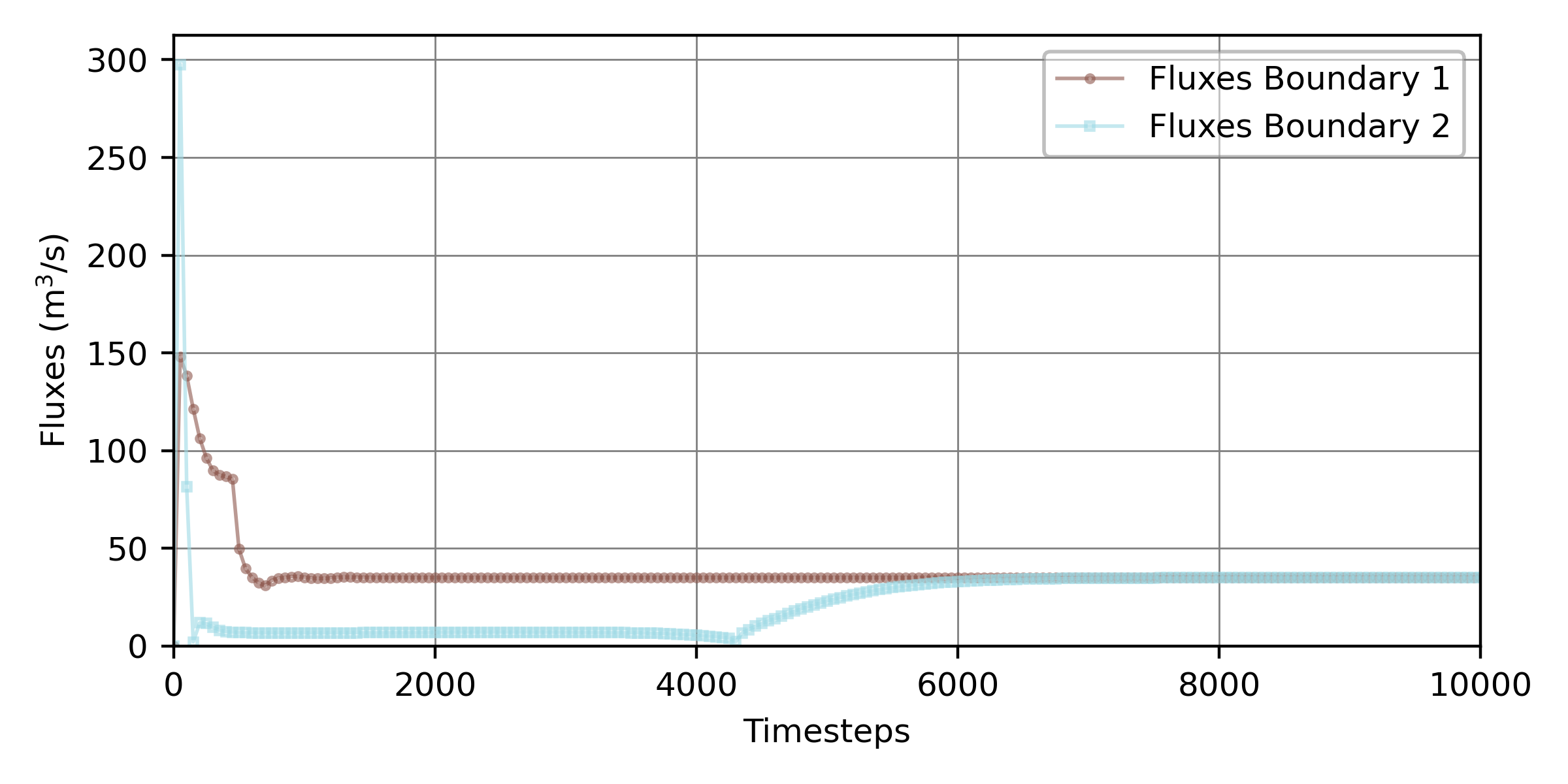
python telemac flux discharge convergence pythomac — Figure 1:Flux convergence plot across the two boundaries of the dry-initialized steady Telemac2d simulation with a total simulation time of timesteps seconds, created with the pythomac.extract_fluxes() function.

Identify Convergence¶

To test if and when the fluxes converged, we track the relative flux imbalance for every timestep $t$ as:

\varepsilon_{t} = \frac{\left| |Q_{i,t}| - |Q_{j,t}| \right|}{|Q_{j,t}|}

(1)

where $Q_{i,t}$ and $Q_{j,t}$ are the outflow and inflow fluxes across the model boundaries at timestep $t$ , respectively. The flux magnitudes $|\cdot|$ are used because Telemac reports boundary fluxes with a sign (inflow positive, outflow negative); mass balance then corresponds to $|Q_{i,t}| = |Q_{j,t}|$ , so that $\varepsilon_{t} \to 0$ at convergence, and normalizing by the inflow $|Q_{j,t}|$ makes $\varepsilon_{t}$ dimensionless. In a stable steady simulation, the ratio of consecutive flux imbalances should converge toward a convergence constant $c_{\varepsilon}$ equal to unity with increasing time:

\lim_{t\to \infty} \frac{\varepsilon_{t+1}}{\varepsilon^{\iota}_{t}} = c_{\varepsilon}

(2)

The combination of the convergence rate (or order) $\iota$ , and the convergence constant $c_{\varepsilon}$ indicate:

linear convergence if $\iota$ = 1 and $c_{\varepsilon} \in ]0, 1[$
slow sublinear convergence if $\iota$ = 1 and $c_{\varepsilon}$ = 1
fast superlinear convergence if $\iota$ > 1 and $c_{\varepsilon} \in ]0, 1]$
divergence convergence if $\iota$ = 1 and $c_{\varepsilon}$ > 1; or $\iota$ < 1

Calculate

\varepsilon_{t+1}

To calculate $\varepsilon_{t+1}$ (epsilon_t1) from $\varepsilon_{t}$ (epsilon_t0), we simply roll $\varepsilon_{t}$ by one element in Python:

epsilon_t0 = epsilon[:-1]  # cut off last element
epsilon_t1 = epsilon[1:]   # cut off element zero

To determine the timestep at which a steady simulation can be considered to have reached a stable state, we want to observe when $\iota$ = 1 and $c_{\varepsilon}$ = 1 indicate sublinear convergence. That is, we look for the timestep $t$ above which each additional timestep $t+1$ only insignificantly improves the model precision (read more on the term insignificant in the below section). Thus, assuming that the model convergences in any form, we can set $c_{\varepsilon}$ = 1 to compute $\iota (t)$ as a function of $\varepsilon_{t}$ and $\varepsilon_{t+1}$ :

\begin{align} \frac{\varepsilon_{t+1}}{\varepsilon^{\iota(t)}_{t}} &=c_{\varepsilon} & \Leftrightarrow \\ \iota(t) &= \frac{1}{c_{\varepsilon}} \cdot \log_{\varepsilon_{t}\varepsilon_{t+1}} & \overbrace{\Longleftrightarrow }^{c_{\varepsilon} = 1}\\ \iota(t) &= \log_{\varepsilon_{t}\varepsilon_{t+1}} & \end{align}

(3)

This equation can be implemented in a Python function as follows:

import numpy as np
import pandas as pd


def calculate_convergence(Q_in, Q_out, conv_constant=1.):
    # relative flux imbalance epsilon_t = ||Q_in| - |Q_out|| / |Q_in|; the magnitudes |.|
    #   are needed because Telemac reports outflow negative, so that balance -> epsilon -> 0
    epsilon = np.abs(np.abs(Q_in) - np.abs(Q_out)) / np.abs(Q_in)
    # derive epsilon at t and t+1
    epsilon_t0 = epsilon[:-1]  # cut off last element
    epsilon_t1 = epsilon[1:]   # cut off element zero
    # return the relative imbalance and the convergence rate iota as a pandas DataFrame
    return pd.DataFrame({
        "Relative imbalance": epsilon_t1,
        "Convergence rate": np.emath.logn(epsilon_t0, epsilon_t1) / conv_constant,
    })

To calculate $\iota (t)$ (Python variable name: iota_t) with the above function, amend the example_flux_convergence.py Python script:

# example_flux_convergence.py

# ...
# add to header (alternatively copy-paste the above function into this script):
from pythomac import calculate_convergence

# calculate fluxes_df (see above code block)
fluxes_df = [...]

# calculate iota (t) with the calculate_convergence function
iota_t = calculate_convergence(
    fluxes_df["Fluxes Boundary 1"][1:],  # remove first zero-entry
    fluxes_df["Fluxes Boundary 2"][1:],  # remove first zero-entry
)

The resulting convergence rate $\iota (t)$ is plotted in Fig. 2 for the steady 2d tutorial, with the modified printout periods of 50 seconds and a total simulation time of 10000 seconds.

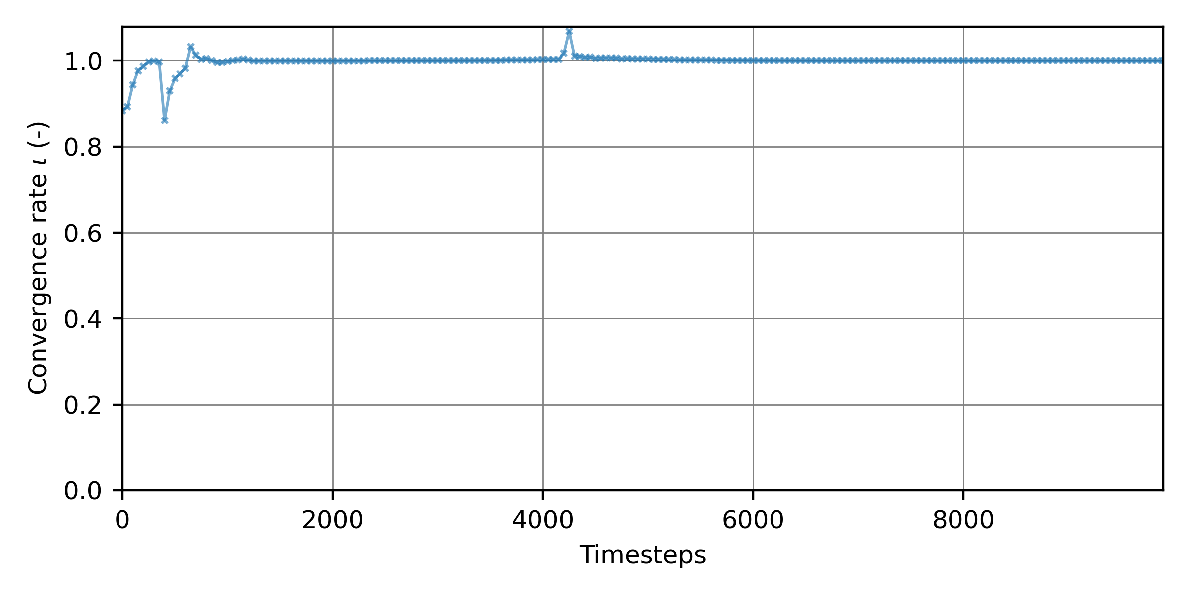
convergence rate fluxes telemac boundaries — Figure 2:The convergence rate $\iota$ as a function 10000 simulation timesteps of the steady 2d simulation.

Derive Optimum Simulation Time¶

To save computing time, we are interested in the timestep at which the inflow and outflow fluxes converged. The fluxes plotted in Fig. 1, and the convergence rate in Fig. 2 qualitatively suggest that the simulation was stable after approximately 6000 seconds (timesteps). The bumps in both figures after 4000 timesteps well indicate the “encounter” of the flux “waves” coming from the upstream and downstream boundaries (see the animation in the steady 2d tutorial). Only afterward, did convergence set in.

The definition of when convergence is reached can be subjective. To save computing time, we look for the smallest timestep $t$ beyond which the relative flux imbalance $\varepsilon_{t}$ (Equation (1)) stays permanently below a target tolerance $\varepsilon_{tar}$ . Tolerances of $\varepsilon_{tar}$ = 10 $^{-4}$ are typically acceptable for preliminary calibration runs, while validation and hotstart-initialization runs warrant smaller values (10 $^{-6}$ or smaller). As Fig. 2 illustrates, the imbalance may briefly drop below the tolerance and rise again after approximately 4000 timesteps, when the upstream “wave” rolls over the downstream boundary; only the last permanent crossing counts. Therefore, we want an algorithmic implementation that detects the last timestep at which $\varepsilon_{t} \geq \varepsilon_{tar}$ and takes the next one as the convergence time. To this end, we can add to the above-started example_flux_convergence.py Python script the following code:

# example_flux_convergence.py

# ...

# calculate fluxes_df (see above code block)
fluxes_df = [...]

# calculate iota_t with calculate_convergence (also returns a "Relative imbalance" column)
iota_t = [...]

# define a desired target tolerance (epsilon_tar) for the relative flux imbalance
target_convergence_precision = 1.0E-4

# get the relative flux imbalance epsilon_t (Delta_Q) from calculate_convergence
relative_imbalance = iota_t["Relative imbalance"].to_numpy()

# find the index of the last element that still exceeds the target tolerance and add +1
#   (i.e., the first element from which the imbalance stays permanently below the tolerance)
below_tolerance = relative_imbalance < target_convergence_precision
idx = np.flatnonzero(~below_tolerance)[-1] + 1

# print the timestep at which the desired convergence was achieved to the console
printout_period_in_cas = 50  # the printout period defined in the cas file
print("The simulation converged after {0} simulation seconds ({1}th printout).".format(
        str(printout_period_in_cas * idx), str(idx)))

The simulation converged after 6000 simulation seconds (120th printout).

Bolster your code

The code for calculating the timestep at which a target convergence level was achieved is also implemented in the get_convergence_time() function in pythomac:

from pythomac import get_convergence_time

A full implementation with also a convenient way for retrieving the printout_period_in_cas variable can be found in this version of example_flux_convergence.py with documentation on https://pythomac.readthedocs.io.

Now that you know when your Telemac simulation converges satisfactorily, you can reduce the NUMBER OF TIME STEPS parameter in the .cas steering file, for example:

/ steady2d-conv.cas
TIME STEP : 1.
NUMBER OF TIME STEPS : 6000
GRAPHIC PRINTOUT PERIOD : 50
LISTING PRINTOUT PERIOD : 50

Troubleshoot Instabilities & Divergence¶

If a steady simulation never reaches stability of fluxes or even flux divergence, make sure that all boundaries are robustly defined according to the spotlight section on boundary conditions, and have a look at the workflow in the next section on mass conservation.