In this section, we will cover fundamental concepts of non-linear classification by introducing the concept of kernels. First, let us recall what we have seen so far in our section about Lineare Klassifizierung. In linear classification, our task consisted of classifying data points through a hyperplane that could linearly separate the dataset in the features coordinate space. For instance, in a 3d feature space, thus a feature vector such as (x1,x2,x3)∈R3, recall that our data is considered linearly separable if there is at least one plane (not line) who can split the points. Unlike linear classification, which assumes a linear relationship between input features and class labels, non-linear classification algorithms use various techniques to capture complex patterns and decision boundaries in the data. In particular, we will look at how we can transform our data into a new coordinate space of higher dimension through kernels, which help us turning the non-linear problem into a linear one.
Kernel ermöglichen es uns, Daten in einen höherdimensionalen Merkmalsraum zu transformieren, in dem eine lineare Trennung möglich wird. Ein Beispiel für einen ML-Algorithmus, der auf Kernel angewiesen ist, um komplexe Muster und Entscheidungsgrenzen in den Daten zu finden, ist Support Vector Machine (SVM).
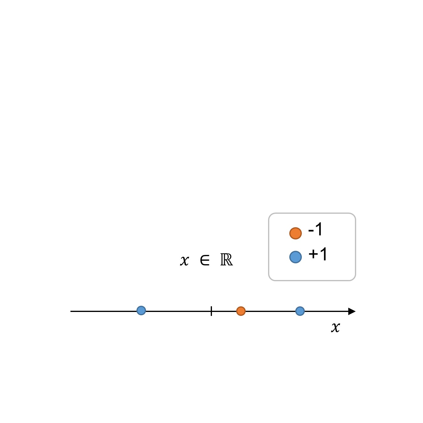
We will now see how feature transformation works through a 1d example, that is, we have one feature x∈R. The figure below illustrates the training points (n=3).
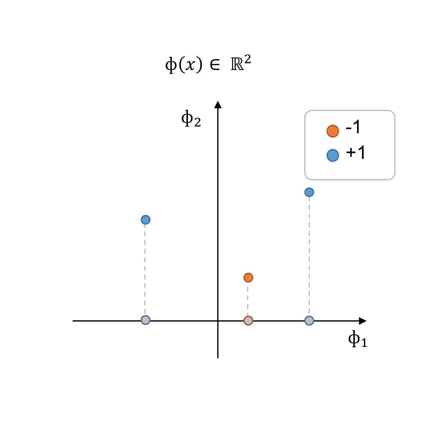
Beachten Sie aus der Abbildung, dass der Datensatz nicht linear trennbar ist, zumindest nicht im angegebenen Merkmalsraum in 1 Dimension. Um dieses Problem in ein lineares Problem zu verwandeln, können wir eine Merkmalstransformation (ϕ(x)) durchführen, um nach einer Entscheidungsgrenze in einem höherdimensionalen Raum zu suchen. Beachten Sie in diesem Beispiel, dass wir das 1D-Feature in einen neuen 2D-Feature-Vektor umwandeln können, wobei die zusätzliche Dimension als eine Art neues Feature angesehen werden kann.
Figure 1:1: Trainingsdaten im ersten Feature Space.
Figure 2:2: Trainingsdatensatz im neuen Feature Space Φ(x).
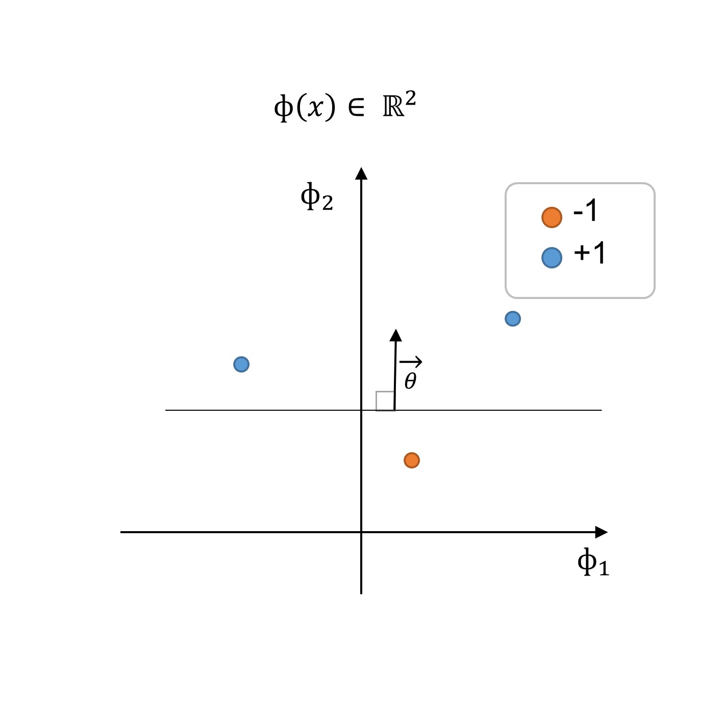
Figure 3:3: Trainingsdatensatz und Entscheidungsgrenze im neuen Feature Space Φ(x)
By performing feature transformation as illustrated in the step 2: training dataset in the new feature space Φ(x) (see figure above), we can find a classifier h(x,θ,θo) with a decision boundary defined by θ and the offset parameter θ0: