Lineare Klassifikation
In diesem Abschnitt werden wir die Grundlagen der linearen Klassifizierung durch einen einfachen ML-Algorithmus, das Perceptron, behandeln. Darüber hinaus werden wir die Konzepte hinter dem Perceptron-Algorithmus erweitern, indem wir Aspekte der *Regularisierung * berücksichtigen, um einen linearen Margin-Klassifikator zu erstellen.
Hyperflugzeuge
Angenommen, wir möchten positive und negative Objekte aus dem Trainingssatz unten klassifizieren (Abbildung links):
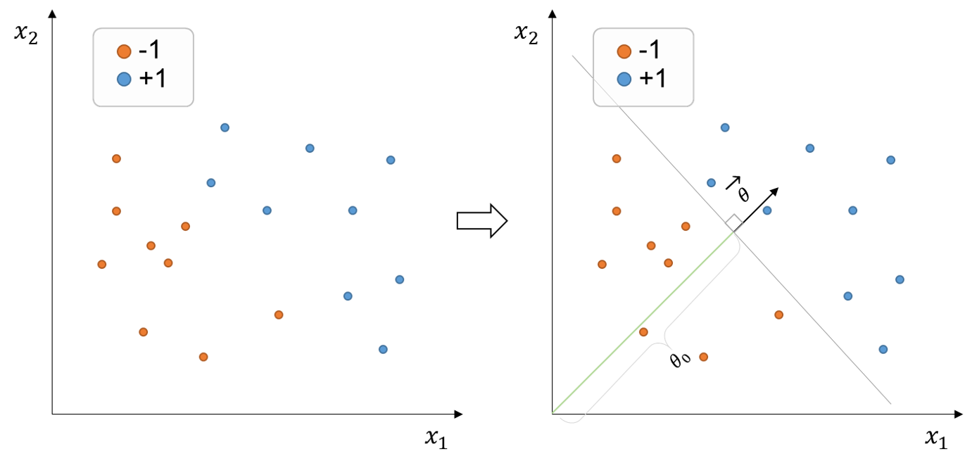
Figure 1:Training set of points with binary labels (+1, -1) and two-dimensional features. The decision boundary (grey line) is defined by the parameter vector , which is normal to the decision boundary, and offset parameter that linearly separates the data.
Der obige Datensatz wird als linear trennbar angesehen, da er mindestens eine lineare Entscheidungsgrenze existiert, die in der Lage ist, den gesamten Datensatz korrekt aufzuteilen. Zum Beispiel könnten wir eine Entscheidungsgrenze wie die graue Linie oben (Abbildung rechts) überschreiten.
In this case, since the features , that is, the feature set belongs to the two-dimensional space, the decision boundary constitutes a line. If we were dealing with a set of features in the three-dimensional space , the decision boundary would be a plane. Analogously, if our feature set were in a higher-dimensional space, the decision boundary would constitute a hyperplane.
A hyperplane with dimensions is conventionally denoted by the vector normal to the plane, , and offset (scalar) parameter . In the example above, we would define the hyperplane (or decision boundary) as:
Unser Klassifikator ist somit gleich , wobei und . Erinnern Sie sich an die Zeichenfunktion, auch bekannt als Signum-Funktion, ist eine mathematische Funktion, die das Zeichen oder die Richtung einer reellen Zahl zurückgibt. Das heißt, wenn die Eingabenummer positiv, negativ oder 0 ist, gibt die Vorzeichenfunktion +1, -1 bzw. 0 zurück.
Perceptron-Algorithmus
In the perceptron algorithm, we typically initialize as zero (zero vector) and loop through the pair of training examples. At every iteration, we will check if the classifier makes a mistake classifying that training example (i-th example), and if so, then we update the parameters of .
Assume that for simplicity (the decision boundary must pass through the origin). Our perceptron classifier will make a mistake if . We will then update our to no longer misclassify that training example. The way to do this is by adding to the previous . Thus, the update would look like:
We have in hands a set of different training examples which have the potential to nudge/update our classifier in many directions. Thus, it is possible and even expected that the last training examples cause updates that will overwrite earlier, initial updates. This will result that earlier examples will no longer be correctly classified. For this reason, we need to loop through the whole training set multiple times to ensure that all examples are correctly classified. Such iterations can be performed both in order or randomly selected from the training examples.
Wir können den Algorithmus wie folgt codieren:
import numpy as np


# Algorithm always starting to loop from x1
def perceptron(X, y, theta, t_times):
    n_mistakes = 0

    # Initialize list to show the progress (updates) of theta
    progress_theta = []

    # Initialize an array with same size as the total number of examples to count how many mistake are made at each training example
    explicit_mistakes = np.zeros(shape=y.shape[0])

    # Loop through the training set T times
    for t in t_times:

        # Loop through the training examples in order
        for index, x in enumerate(X):

            # Check if the algorithm makes a mistake in the i-th (or index-th) example
            if y[index] * np.dot(theta, x) <= 0:
                # Update theta to no longer misclassify the i-th example
                theta = theta + y[index] * x

                # Save the update theta
                progress_theta.append(theta)

                # Update total number of mistakes
                n_mistakes += 1

                # Update total number of mistakes at the i-th training example
                explicit_mistakes[index] += 1
    print('The perceptron did {} mistakes until convergence'.format(n_mistakes))
    return progress_theta, n_mistakes, explicit_mistakes


if __name__ == '__main__':
    X = np.array([[-1, -1], [1, 0], [-1, 1.5]])
    # X = np.array([[-1, -1], [1, 0], [-1, 10]])

    y = np.array([1, -1, 1])

    t_times = range(0, 100)

    theta = np.array([-1, -1])

    a, b, c = perceptron(X, y, theta, t_times)
Margin-Grenzen und Scharnierverlust
Wie Sie vielleicht bemerkt haben, verfügt der Perceptron-Algorithmus über keinen Regularisierungsbegriff. Das Ziel war einfach, eine Entscheidungsgrenze zu finden, die die Daten korrekt aufteilen kann. Hier werden wir das Konzept von *Hindernisverlust * und *Margengrenzen * vorstellen, um das Problem des Erlernens einer Entscheidungsgrenze in ein Optimierungsproblem unter Berücksichtigung der Regularisierung zu verwandeln.
Motivation hinter Margengrenzen
Werfen wir einen Blick auf unseren zuvor vorgestellten Trainingsdatensatz (Abbildung unten). Jede Entscheidungsgrenze innerhalb der gestrichelten grauen Linien teilt die Trainingsbeispiele korrekt auf. Wir möchten jedoch intuitiv eine Entscheidungsgrenze bevorzugen, die die Abstände zwischen der Entscheidungsgrenze und den Trainingspunkten maximieren kann. Der Grund dafür ist, dass die Punkte, die wir in Zukunft klassifizieren möchten, wahrscheinlich ein statistisches Rauschen haben, so dass eine Entscheidungsgrenze, die zu nahe an den Trainingsbeispielen liegt, eher leicht veränderte (lautere) Versionen der Trainingsbeispiele falsch klassifiziert. Im Gegensatz dazu wird ein Klassifikator, der eine relativ höhere Marge zwischen der Entscheidungsgrenze und den Beispielen hat, wahrscheinlich erfolgreicher bei der Klassifizierung zukünftiger, unsichtbarer Daten sein.
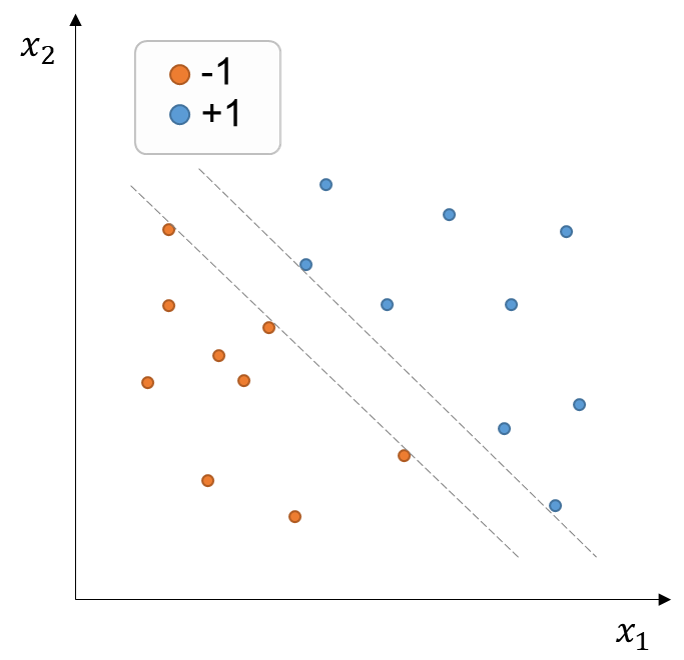
Figure 3:Trainingssatz von Punkten mit binären Labels (+1, -1) im zweidimensionalen Feature Space . Jede Entscheidungsgrenze innerhalb der gestrichelten grauen Linien kann die Daten korrekt aufteilen.
Optimierungsproblem
Denken Sie daran, dass es unser Ziel ist, einen linearen Klassifikator zu finden, der die Abstände zwischen der Entscheidungsgrenze und den Trainingspunkten maximiert (margin linearer Klassifikator), aber auch den Trainingsfehler minimiert. Dies stellt somit ein Optimierungsproblem dar, das diese beiden Faktoren ausgleichen muss, die wir als Folgendes angeben können:
Die Margen (Abstände zwischen der Entscheidungsgrenze und den Trainingspunkten) sollten maximiert werden.
Der Trainingsfehler sollte minimiert werden. Wir werden dies als *Hindernisverlust * ausdrücken.
Grenzgrenzen
Previously, we saw that the equation defining a decision boundary satisfies .
Wir können nun parallele Randgrenzen (gestrichelte Linie in der vorherigen Abbildung) als definieren:
Note that we can define the boundaries like this because we have a degree of freedom in our definition of the decision boundary, namely, the magnitude of the normal vector . That is, regardless of the value , our decision boundary remains unaltered.
Erinnern Sie sich an das Problem der Berechnung der kleinste Abstand eines Punktes zu einem Flugzeug]. Dieser Abstand beträgt:
Wir können nun den signierten Abstand zwischen der Entscheidungsgrenze und dem i-ten Beispiel berechnen als:
Der Abstand zwischen den Randgrenzen und der Entscheidungsgrenze beträgt somit:
Gelenkverlust
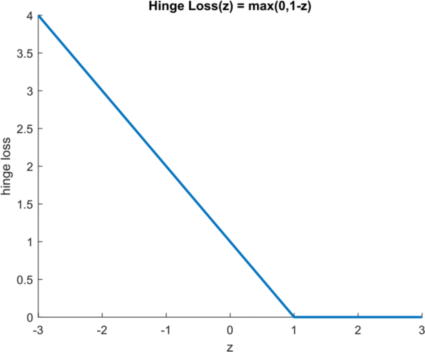
We so far know that will classify the i-th example. The way to know if the classification agrees with the label is by multiplying it by . We can express this agreement also in a slightly modified version, using the hinge loss:
Dabei ist die Vereinbarung (signierte Entfernung von der Entscheidungsgrenze) .
Die folgende Abbildung zeigt, wie der Scharnierverlust entlang der z-Achse (Abstand von der Grenze) funktioniert, wie in dieser ResearchGate-Publikation] gezeigt:
Zielfunktion
So now we can create an objective function that (1) minimizes the average hinge loss over the training examples, and (2) maximizes . Expression (2) can be also reformulated towards minimizing . Thus we define the objective function as:
where is the regularization parameter that balances the importance of minimizing the regularization term at the cost of incurring more losses (increasing the loss term). Vice versa, the smaller the value of , the more emphasis we will give to minimizing average loss.