Get ready by cloning the exercise repository:
git clone https://github.com/Ecohydraulics/Exercise-geco.gitSacramento suckers in the South Yuba River (source: Sebastian Schwindt @hydroinformatics on YouTube).
What is Habitat Suitability?
Fish and other aquatic species rest, orient, and reproduce in a fluvial environment that represents their physical habitat. Throughout their different life stages, different fish have specific physical habitat preferences which are defined, for instance, as a function of water depth, flow velocity, and grain size of the riverbed. The so-called Habitat Suitability Index can be calculated for hydraulic (water depth or flow velocity) and morphological (e.g., grain size or cover in the form of large wood) parameters individually to describe the quality of physical habitat for a fish and at a specific life stage. The figure below shows exemplary curves for the fry, juvenile, and adult life stages of rainbow trout as a function of water depth. The curves look different in every river and should be established individually by an aquatic ecologist.
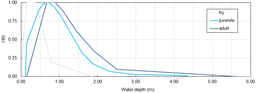
Figure 1:Habitat Suitability Index curves for the fry, juvenile, and adult life stages of rainbow trout in a cobble-bed river. Take care: HSI curves look different in any river and need to be established by an aquatic ecologist.
The concept also accounts for the so-called cover habitat in the form of the cover Habitat Suitability Index . Cover habitat is the result of local turbulence caused by roughness elements such as wood, boulders, or bridge piers. However, in this exercise, we will only deal with hydraulic habitat characteristics (not cover habitat).
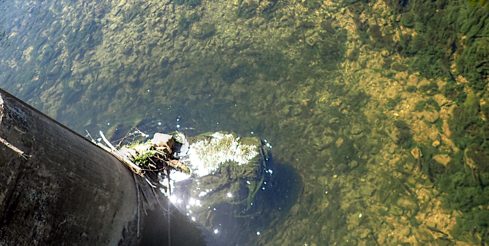
Adult trout swimming in cover habitat created by a bridge pier in the upper Neckar River.
The combination of multiple values (e.g., water depth-related , flow velocity-related , grain size-related , and/or cover ) results in the combined Habitat Suitability Index . There are various calculation methods for combining different values into one value, where the geometric mean and the product are the most widely used deterministic combination methods:
Therefore, if the pixel-based values for water depth and flow velocity are known from a two-dimensional (2d) hydrodynamic model, then for each pixel the value can be calculated either as the product or geometric mean of the single-parameter rasters.
This habitat assessment concept was introduced by Bovee (1986) and Stalnaker et al. (1995) (direct download). However, these authors built their usable (physical) habitat assessment based on one-dimensional (1d) numerical models that were commonly used in the last millennium. Today, 2d numerical models are the state-of-the-art to determine physical habitat geospatially explicit based on pixel-based values. There are two different options for calculating the usable habitat area () based on pixel-based values (and even more options can be found in the scientific literature).
An alternative to the deterministic calculation of the and values of a pixel is a fuzzy logic approach Noack et al., 2013. In the fuzzy logic approach, pixels are classified, for instance, as low, medium, or high habitat quality as a function of the associated water depth or flow velocity using categorical (low, medium, or high), expert assessment-based curves. The value results from the center of gravity of superimposed membership functions of considered parameters (e.g., water depth and flow velocity).
Sustainable river management involves the challenge of designing an aquatic habitat for target fish species at different life stages. The concept of usable physical habitat area represents a powerful tool to leverage the assessment of the ecological integrity of river management and engineering measures. For example, by calculating the usable habitat area before and after the implementation of measures, valuable conclusions can be drawn about the ecological integrity of restoration efforts.
This exercise demonstrates the use of 2d hydrodynamic modeling results to algorithmically evaluate usable habitat area based on the calculation of geospatially explicit values.
Available Data and Code Structure
The following flow chart illustrates the provided code and data. Functions, methods, and files to be created in this exercise are highlighted in bold, italic, YELLOW-ish font.
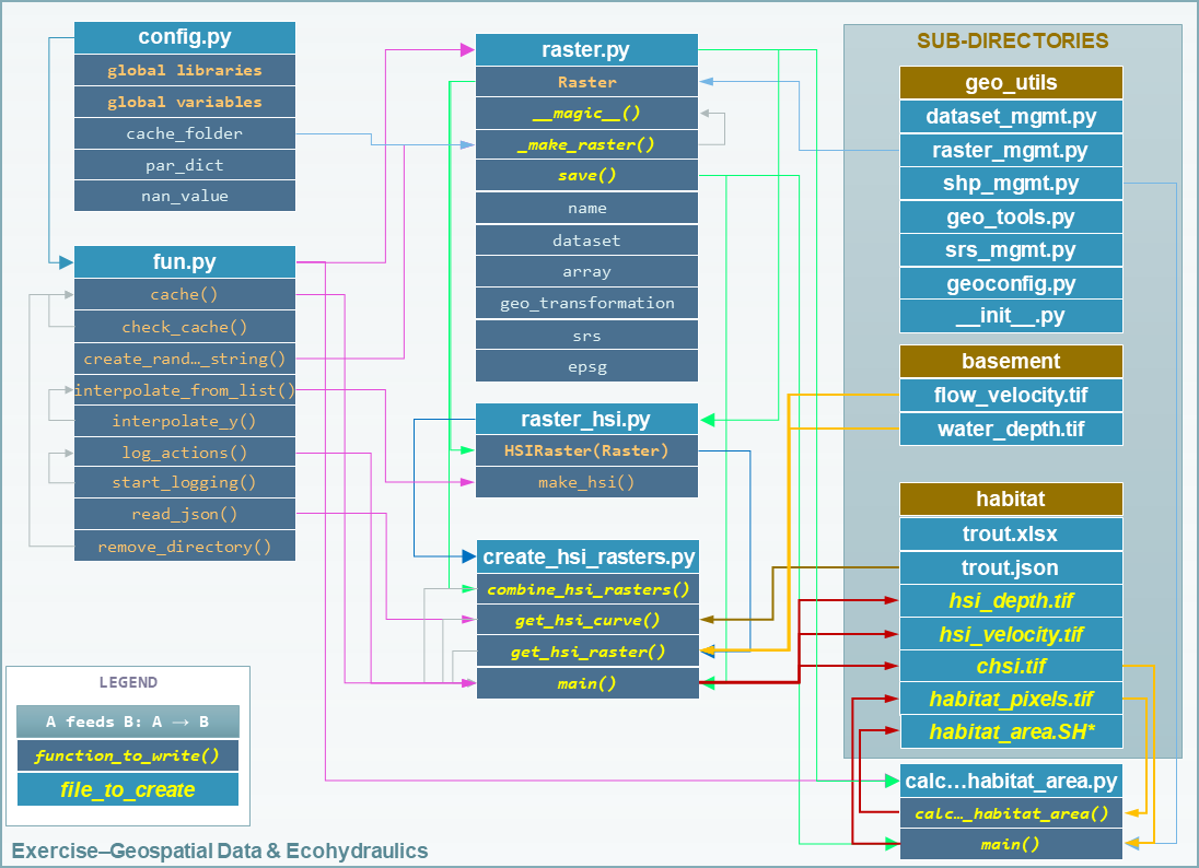
Figure 2:Structure of the provided template file tree and their relations.
The provided QGIS project file visualize_with_QGIS.qgz helps to verify input raster datasets and results.
Two-dimensional (2d) Hydrodynamic Modelling (Folder: BASEMENT)
This exercise uses (hydraulic) flow velocity and water depth rasters (GeoTIFFs) produced with the ETH Zurich*s BASEMENT software. Read more about hydrodynamic modeling with BASEMENT in the BASEMENT chapter. The hydraulic rasters were produced with the BASEMENT developer’s example data from the Flaz River in Switzerland (read more on their website).
The water depth water_depth.tif and flow velocity flow_velocity.tif rasters are provided for this exercise in the folder /basement/.
Habitat Suitability Index HSI Curves (folder: habitat)
The /habitat/ folder in the exercise repository contains curves in the form of an xlsx workbook (trout.xlsx) and in the form of a JSON file (trout.json). Both files contain the same data for rainbow trout of a hypothetical cobble-bed river and this exercise only uses the JSON file (the workbook serves for visual verification only).
Code
Create and Combine HSI Rasters
Complete the __init__ Method of the Raster Class (raster.py)
The raster.py script imports the functions and libraries loaded in the fun.py script, and therefore, also the config.py script. For this reason, the NumPy and Pandas libraries are already available (as np and pd, respectively), and the geo_utils package is already imported as geo (import geo_utils as geo in config.py).
The Raster class will load any GeoTIFF file name as a geo-referenced array object that can be used with mathematical operators. First, we will complement the __init__ method by a Raster.name (extract from the file_name argument), as well as georeferences and array datasets:
    # __init__(...) of Raster class in raster.py
        self.name = file_name.split("/")[-1].split("\\")[-1].split(".")[0]
If the provided file_name does not exist, the __init__ method creates a new raster with the file_name (this behavior is already implemented in the if not os.path.exists(file_name) statement.
Next, load the osgeo.gdal.dataset, the np.array, and the geo_transformation of the raster. For this purpose, use the raster2array function from this eBook, which is also implemented in the exercise’s geo_utils (geo) package:
    # __init__(...) of Raster class in raster.py
        self.dataset, self.array, self.geo_transformation = geo.raster2array(file_name, band_number=band)
To identify the EPSG number (Authority code) of a raster, retrieve the spatial reference system (SRS) of the raster. Also for this purpose we have already developed a function in the lecture with the get_srs from the theory section on reprojection. Load the SRS and the EPSG number using the get_srs function with the following two lines of code in the __init__ method:
    # __init__(...) of Raster class in raster.py
        self.srs = geo.get_srs(self.dataset)
        self.epsg = int(self.srs.GetAuthorityCode(None)
The __init__ method of the Raster class is complete.
Complete Magic Methods of the Raster Class (raster.py)
To enable mathematical operations between multiple instances of the Raster class, implement Overloading and Magic Methods that tell the class what to do when two Raster instances are for example added (+ sign), multiplied (* sign), or subtracted (- sign). For instance, implementing the magic methods __truediv__ (for using the / operator), __mul__ (for using the * operator), and __pow__ (for using the ** operator) will enable the usage of Raster instances like this:
# example for Raster instances, when operators are defined through magic methods

# load GeoTIFF rasters from file directory
velocity = Raster("/usr/geodata/u.tif")
depth = Raster("/usr/geodata/h.tif")

# calculate the Froude number using operators defined with magic methods
Froude = velocity / (depth * 9.81) ** 0.5

# save the new raster
Froude.save("/usr/geodata/froude.tif")
The Raster class template already contains one exemplary magic method to enable division (__truediv__):
    # Raster class in raster.py
    def __truediv__(self, constant_or_raster):
        try:
            self.array = np.divide(self.array, constant_or_raster.array)
        except AttributeError:
            self.array /= constant_or_raster
        return self._make_raster("div")
Here is what the __truediv__ method does:
The input argument
constant_or_rastercan be anotherRasterinstance that has anarrayattribute or a numeric constant (e.g., 9.81).The method tries to invoke the array attribute of
constant_or_raster.If
constant_or_rasteris a raster object, then invokingcontant_or_raster.arrayis successful. In this caseself.arrayis overwritten with the element-wise division of the array bycontant_or_raster.array. The element-wise division builds on NumPys built-in function np.divide, which is a computationally efficient wrapper of C/C++ code (much faster than a Python loop over array elements).If
constant_or_rasteris a numeric value, then invokingcontant_or_raster.arrayresults in anAttributeErrorand the__truediv__method falls in theexcept AttributeErrorstatement, whereself.arrayis simply divided byconstant_or_raster.
The method returns the result of the pseudo private method
self._make_raster("div")([recall PEP 8 Code Style and Conventions, which corresponds to a newRasterinstance of the actualRasterinstance divided byconstant_or_raster. The newRasterinstance is a temporary GeoTIFF file in the cache folder (recall the cache function). This is how the pseudo-private method_make_raster(self, file_marker)looks like:
This function:
Uses the string-type argument
file_markerto add it to the file name of the base GeoTIFF along with a random, four characters-long string (recall the create_random_string).file_markeris unique for every implemented operator. For the__truediv__method usefile_marker="div". Thus, the temporary GeoTIFF file name is defined ascache_folder + self.name + f_ending(e.g."C:\Excercise-geco\__cache__\velocity__divhjev__.tif").Applies the Create a Raster (Array to Raster) function from
geo_utilsto write the temporary GeoTIFF to the__cache__folder with the original raster’s spatial reference system.returns a newRasterinstance of the temporary, cached GeoTIFF file.
If you find the _make_raster method confusing...
Then you have a point. The above-described approach implements the _make_raster method to reuse the temporary GeoTIFFs later with both constants (float) and arrays, but there is a more elegant way to return a new Raster instance. However, returning a new instance of the same class requires that the input argument must be an instance of the class itself (i.e., Raster) and not a numeric variable. The alternative solution for returning a Raster instance starts with a different implementation of the magic method (e.g., __truediv__) and requires importing Python4-style annotations. Therefore, the first line of the script must include (only works with Python 3.7 and higher) the following import:
from __future__ import annotationsThen rewrite the __truediv__ method:
    def __truediv__(self, other: Raster) -> Raster:
        f_ending = "__div%s__.tif" % create_random_string(4)
        return Raster(file_name=cache_folder + self.name + f_ending,
                      raster_array=np.divide(self.array, other.array),
                      epsg=self.epsg,
                      geo_info=self.geo_transformation)
In this case, the _make_raster method is obsolete. Read more about returning instances of the same class on stack overflow.
When using the _make_raster method, add the following magic methods to the Raster class (function placeholders are already present in the raster.py template):
__add__(+operator):
        try:
            self.array += constant_or_raster.array
        except AttributeError:
            self.array += constant_or_raster
return self._make_raster("add")__mul__(*operator):
        try:
            self.array = np.multiply(self.array, constant_or_raster.array)
        except AttributeError:
            self.array *= constant_or_raster
return self._make_raster("mul")__pow__(**operator):
        try:
            self.array = np.power(self.array, constant_or_raster.array)
        except AttributeError:
            self.array **= constant_or_raster
return self._make_raster("pow")__sub__(-operator):
        try:
            self.array -= constant_or_raster.array
        except AttributeError:
            self.array -= constant_or_raster
        return self._make_raster("sub")
The last item to complete in the Raster class is the built-in save method that receives a file_name (string) argument defining the directory and save-as name of the Raster instance:
        save_status = geo.create_raster(file_name, self.array, epsg=self.epsg, nan_val=0.0, geo_info=self.geo_transformation)
        return save_status
Why do we need the save_status variable? First, it states if saving the raster was successful (save_status=0), and second, this information could be used to delete the raster from the __cache__ folder and flush the memory (feel free to do so for speeding up the code).
Write HSI and cHSI Raster Creation Script
The provided create_hsi_rasters.py script already contains required package imports, an if __name__ == '__main__' stand-alone statement as well as the void main, get_hsi_curve, get_hsi_raster, and combine_hsi_rasters functions:
The if __name__ == '__main__' statement contains a time counter (perf_counter) that prompts how long the script takes to run (typically between 3 to 6 seconds). Make sure that
the
parameterslist contains"velocity"and"depth"(as per thepar_dictin theconfig.pyscript),the file paths are defined correctly, and
a life stage is defined (i.e., either
"fry","juvenile","adult", or"spawning"as per the /habitat/fish.xlsx workbook).
The following paragraphs show step by step how to load the curves from the JSON file (get_hsi_curve), apply them to the flow_velocity and water_depth rasters (get_hsi_raster), and combine the resulting rasters into rasters (combine_hsi_rasters).
The get_hsi_curve function will load the curve from the JSON file (/habitat/trout.json) in a dictionary for the two parameters "velocity" and "depth". Thus, the goal is to create a curve_data dictionary that contains one Pandas DataFrame object for all parameters (i.e., velocity and depth). For example, curve_data["velocity"]["u"] will be a Pandas Series of velocity entries (in m/s) that corresponds to curve_data["velocity"]["HSI"], which is a Pandas Series of values. Similarly, curve_data["depth"]["h"] is a Pandas Series of depth entries (in meters) that corresponds to curve_data["depth"]["HSI"], which is a Pandas Series of values (corresponds to the curves shown in the HSI graphs above). To extract the desired information from the JSON file, get_hsi_curve takes three arguments (json_file, life_stage, and parameters) in order to:
Get the information stored in the JSON file with the
read_jsonfunction (see above).Instantiate a void
curve_dataDictionary that will contain the PandasDataFrames for"velocity"and"depth".Run a loop over the (two) parameters (
"velocity"and"depth"), in which it:Creates a void
par_pairsList for storing pairs of parameter (par) - values as nested lists.Iterates through the length of provided curve data, where valid data pairs (e.g.,
[u_value, HSI_value]) are appended to thepar_pairsList. This iteration is what actually creates the nested List.Converts the final
par_pairslist to a PandasDataFramethat it adds to thecurve_dataDictionary.
returnthecurve_dataDictionary with its PandasDataFrames.
# create_hsi_rasters.py
def get_hsi_curve(json_file, life_stage, parameters):
    # read the JSON file with fun.read_json
    file_info = read_json(json_file)
    # instantiate output dictionary
    curve_data = {}
    # iterate through parameter list (e.g., ["velocity", "depth"])
    for par in parameters:
        # create a void list to store pairs of parameter-HSI values as nested lists
        par_pairs = []
        # iterate through the length of parameter-HSI curves in the JSON file
        for i in range(0, file_info[par][life_stage].__len__():
            # if the parameter is not empty (i.e., __len__ > 0), append the parameter-HSI (e.g., [u_value, HSI_value]) pair as nested list
            if str(file_info[par][life_stage][i]["HSI"]).__len__() > 0:
                try:
                    # only append data pairs if both parameter and HSI are numeric (floats)
                    par_pairs.append([float(file_info[par][life_stage][i][par_dict[par]]),
                                      float(file_info[par][life_stage][i]["HSI"])])
                except ValueError:
                    logging.warning("Invalid HSI curve entry for {0} in parameter {1}.".format(life_stage, par)
        # add the nested parameter pair list as pandas DataFrame to the curve_data dictionary
        curve_data.update({par: pd.DataFrame(par_pairs, columns=[par_dict[par], "HSI"])})
    return curve_data
In the main function, call get_hsi_curves to get the curves as a Dictionary. In addition, implement the cache and the log_actions wrappers (recall the descriptions of provided functions) for the main function:
# create_hsi_rasters.py

...

@log_actions
@cache
def main():
    # get HSI curves as pandas DataFrames nested in a dictionary
    hsi_curve = get_hsi_curve(fish_file, life_stage=life_stage, parameters=parameters)

...
With the provided HSIRaster (raster_hsi.py) class, the rasters can be conveniently created in the get_hsi_raster function. Before using the HSIRaster class, make sure to understand how it works. The HSIRaster class inherits from the Raster class and initiates its parent class in its __init__ method through Raster.__init__(self, file_name=file_name, band=band, raster_array=raster_array, geo_info=geo_info). Then, the class calls its make_hsi method, which takes an curve (nested List) of two equal List pairs (List of parameters and List of values) as argument. The make_hsi method:
Extracts parameter values (e.g., depth or velocity) from the first element of the nested
hsi_curvesList, and values from the second element of the nestedhsi_curvesList.Uses NumPys built-in
np.nditerfunction, which iterates through NumPy arrays with high computational efficiency (read more aboutnditer).The
nditerloop passes thepar_valuesasx_valuesList argument and thehsi_valuesasy_valuesList arguments to theinterpolate_from_listfunction (recall the function descriptions above).The array values (i.e., flow velocity or water depth) correspond to the
xi_valuesList argument of theinterpolate_from_listfunction.The
interpolate_from_listfunction then identifies for each element of thexi_valuesList the closest elements ( values) in thex_valuesList and the corresponding positions in they_valuesList.The
interpolate_from_listfunction passes the identified values to theinterpolate_yfunction, which then linearly interpolates the correspondingyivalue (i.e., an value).Thus, the flow velocity or water depths in
self.arrayare row-wise (row-by-row) replaced by values.
returns aRasterinstance using the pseudo-private_make_rastermethod (recall its contents).
# raster_hsi.py
from raster import *

class HSIRaster(Raster):
    def __init__(self, file_name, hsi_curve, band=1, raster_array=None, geo_info=False):
        Raster.__init__(self, file_name=file_name, band=band, raster_array=raster_array, geo_info=geo_info)
        self.make_hsi(hsi_curve)

    def make_hsi(self, hsi_curve):
        par_values = hsi_curve[0]
        hsi_values = hsi_curve[1]
        try:
            with np.nditer(self.array, flags=["external_loop"], op_flags=["readwrite"]) as it:
                for x in it:
                    x[...] = interpolate_from_list(par_values, hsi_values, x)
        except AttributeError:
            print("WARNING: np.array is one-dimensional.")
        return self._make_raster("hsi")
Modify the get_hsi_rasters function to directly return a HSIRaster object:
# create_hsi_rasters.py

...

def get_hsi_raster(tif_dir, hsi_curve):
    return HSIRaster(tif_dir, hsi_curve)
...
The get_hsi_raster function requires two arguments, which it must receive from the main function. For this reason, iterate over the parameters List in the main function and extract the corresponding raster directories from the tifs Dictionary (recall the variable definition in the standalone statement). In addition, save the Raster objects returned by the get_hsi_raster function in another Dictionary (eco_rasters) to combine them in the next step into a raster.
# create_hsi_rasters.py

...

@log_actions
@cache
def main():
    # get HSI curves as pandas DataFrames nested in a dictionary
    hsi_curve = get_hsi_curve(fish_file, life_stage=life_stage, parameters=parameters)

        # create HSI rasters for all parameters considered and store the Raster objects in a dictionary
    eco_rasters = {}
    for par in parameters:
        hsi_par_curve = [list(hsi_curve[par][par_dict[par]]),
                         list(hsi_curve[par]["HSI"])]
        eco_rasters.update({par: get_hsi_raster(tif_dir=tifs[par], hsi_curve=hsi_par_curve)})
        eco_rasters[par].save(hsi_output_dir + "hsi_%s.tif" % par)
...
Of course, one can also loop over the parameters List directly in the get_hsi_raster function.
Next, we come to the reason why we had to define magic methods for the Raster class: combine the rasters using both combination formulae presented above (recall the product and geometric mean formulae), where "geometric_mean" should be used by default. The combine_hsi_rasters function accepts two arguments (a List of Raster objects corresponding to rasters and the method to use as string).
If the method corresponds to the default value "geometric_mean", then the power to be applied to the product of the Raster List is calculated from the nth root, where n corresponds to the number of Raster objects in the raster_list. Otherwise (e.g., method="product"), the power is exactly 1.0.
The combine_hsi_rasters function initially creates an empty Raster in the cache_folder, with each cell having the value 1.0 (filled through np.ones). In a loop over the Raster elements of the raster_list, the function multiplies each raster with the raster.
Finally, the function returns the product of all rasters to the power of the previously determined power value.
# create_hsi_rasters.py
def combine_hsi_rasters(raster_list, method="geometric_mean"):
    if method is "geometric_mean":
        power = 1.0 / float(raster_list.__len__()
    else:
        # supposedly method is "product"
        power = 1.0

    chsi_raster = Raster(cache_folder + "chsi_start.tif",
                         raster_array=np.ones(raster_list[0].array.shape),
                         epsg=raster_list[0].epsg,
                         geo_info=raster_list[0].geo_transformation)
    for ras in raster_list:
        chsi_raster = chsi_raster * ras

    return chsi_raster ** power
To finish the create_hsi_rasters.py script, implement the call to the combine_hsi_rasters function in the main function and save the result as GeoTIFF raster in the /habitat/ folder:
# create_hsi_rasters.py

...

@log_actions
@cache
def main():
    ...

    for par in parameters:
        hsi_par_curve = [list(hsi_curve[par][par_dict[par]]),
                         list(hsi_curve[par]["HSI"])]
        eco_rasters.update({par: get_hsi_raster(tif_dir=tifs[par], hsi_curve=hsi_par_curve)})
        eco_rasters[par].save(hsi_output_dir + "hsi_%s.tif" % par)

    # get and save chsi raster
    chsi_raster = combine_hsi_rasters(raster_list=list(eco_rasters.values(),
                                      method="geometric_mean")
    chsi_raster.save(hsi_output_dir + "chsi.tif")
...
Run the HSI and cHSI Code
A successful run of the script create_hsi_rasters.py should look like this (in PyCharm):
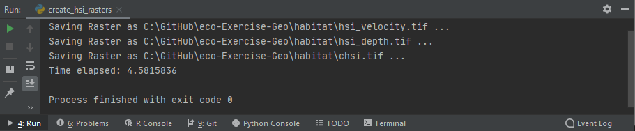
Figure 3:A Windows Python console running the above-created scripts.
Plotted in QGIS, the GeoTIFF raster should look like this:
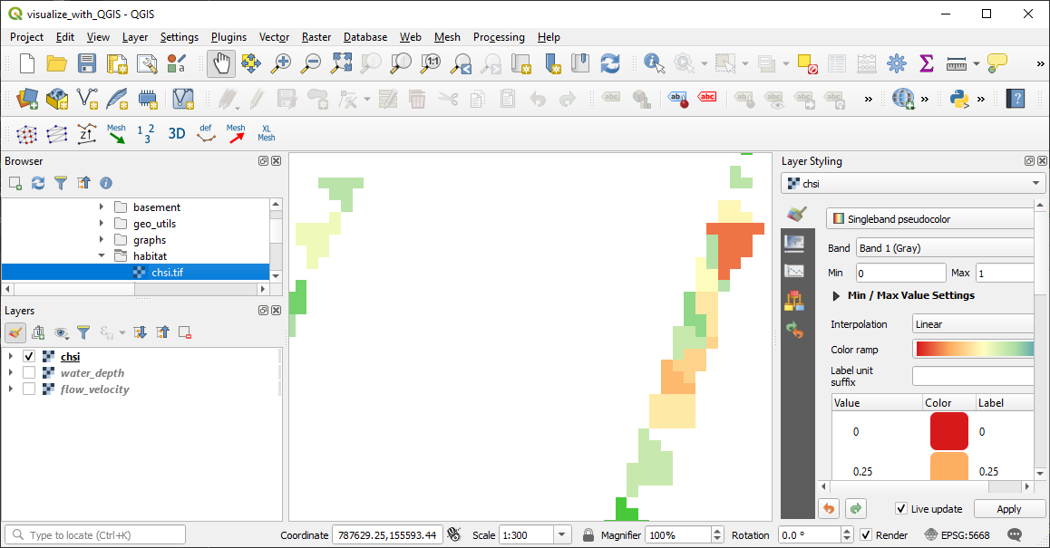
Figure 4:The cHSI raster plotted in QGIS, where poor physical habitat quality (cHSI close to 0.0) is colored in red and high physical habitat quality (cHSI close to 1.0) is colored in green.
Result Interpretation
The presentation of the raster shows that preferred habitat areas for juvenile trout exist only close to the banks. Also, numerical artifacts of the triangular mesh used by BASEMENT are visible. Therefore, the question arises whether the calculated flow velocities and water depths, and in consequence also the values, close to the banks can be considered representative.
Calculate Usable Habitat Area UHA
Write the Code
The rasters enable the calculation of the available usable habitat area. The previous section featured examples using the fish species trout and its juvenile life stage, for which we will determine here the usable habitat area (in m) using a threshold value (rather than the pixel area weighting approach). So we follow the threshold formula described above, using a threshold value of . Thus, every pixel that has a value of 0.4 or greater counts as usable habitat area.
From a technical point of view, this part of the exercise is about converting a raster into a polygon shapefile as well as accessing and modifying the Attribute Table of the shapefile.
Similar to the creation of the raster, there is a template script available for this part of the exercise, called calculate_habitat_area.py, which contains package and module imports, an if __name__ == '__main__' stand-alone statement, as well as the void main and calculate_habitat_area functions. (uha-template)=
The template script looks like this:
# this is calculate_habitat_area.py (template)
from fun import *
from raster import Raster


def calculate_habitat_area(layer, epsg):
    pass


def main():
    pass


if __name__ == '__main__':
    chsi_raster_name = os.path.abspath("") + "\\habitat\\chsi.tif"
    chsi_threshold = 0.4

    main()
In the if __name__ == '__main__' statement, make sure that the global variable chsi_raster_name corresponds to the directory of the raster created in the previous section. The other global variable (chsi_threshold) corresponds to the value of 0.4 that we will use with the threshold formula.
In the main function, start with loading the raster (chsi_raster) as a Raster object. Then, access the NumPy array of the raster and compare it with chsi_threshold using NumPys built-in greater_equal function. np.greater_equal takes an array as first argument and a second argument, which is the condition that can be a numeric variable or another NumPy array. Then, np.greater_equal checks if the elements of the first array are greater than or equal to the second argument. In the case of the second argument being an array, this is an element-wise comparison. The result of np.greater_equal is a Boolean array (True where the greater-or-equal condition is fulfilled and False otherwise). However, to create an osgeo.gdal.Dataset object from the result of np.greater_equal, we need a numeric array. For this reason, multiply the result of np.greater_equal by 1.0 and assign it as a new NumPy array of zeros (False) and ones (True) to a variable named habitat_pixels (see the code block below).
With the habitat_pixels array and the georeference of chsi_raster, create a new integer GeoTIFF raster with the create_raster function (also available in flusstools.geotools); here, use geo.create_raster. In the following code block the new raster is saved in the /habitat/ folder of the exercise as habitat-pixels.tif.
# calculate_habitat_area.py
...

def main():
    # open the chsi raster
    chsi_raster = Raster(chsi_ras_name)
    # extract pixels where the physical habitat quality is higher than the user threshold value
    habitat_pixels = np.greater_equal(chsi_raster.array, chsi_threshold_value) * 1
    # write the habitat pixels to a binary array (0 -> no habitat, 1 -> usable habitat)
    geo.create_raster(os.path.abspath("") + "\\habitat\\habitat-pixels.tif",
                      raster_array=habitat_pixels,
                      epsg=chsi_raster.epsg,
                      geo_info=chsi_raster.geo_transformation)
...
In the next step, convert the habitat pixel raster into a polygon shapefile and save it in the /habitat/ folder as habitat-area.shp. The conversion of a raster into a polygon shapefile requires that the raster contains only integer values, which is the case in the habitat pixel raster (only zeros and ones - recall Raster to Polygon). Use the raster2polygon function in the geo_utils folder (package) to create the new polygon shapefile, specify habitat-pixels.tif as raster_file_name to be converted, and /habitat/habitat-area.shp as output file name. The geo.raster2polygon function returns an osgeo.ogr.DataSource object and we can pass its layer including the information of the EPSG authority code (from chsi_raster) directly to the not-yet-written calculate_habitat_area() function:
# calculate_habitat_area.py
...

def main():
    ... (create habitat pixels raster)

    # convert the raster with usable pixels to polygon (must be an integer raster!)
    tar_shp_file_name = os.path.abspath("") + "\\habitat\\habitat-area.shp"
    habitat_polygons = geo.raster2polygon(os.path.abspath("") + "\\habitat\\habitat-pixels.tif",
                                          tar_shp_file_name)

    # calculate the habitat area (will be written to the attribute table)
    calculate_habitat_area(habitat_polygons.GetLayer(), chsi_raster.epsg)
...
For the calculate_habitat_area() function to produce what its name promises, we need to populate this function as well. For this purpose, use the epsg integer argument to identify the unit system of the shapefile.
# calculate_habitat_area.py
...

def calculate_habitat_area(layer, epsg):
    # retrieve units
    srs = geo.osr.SpatialReference()
    srs.ImportFromEPSG(epsg)
    area_unit = "square %s" % str(srs.GetLinearUnitsName()
...To determine the habitat area, the area of each polygon must be calculated. For this purpose, add a new field to the layer in the Attribute Table, name it "area", and assign a geo.ogr.OFTReal (numeric) data type (recall how to create a field an data types).
Then, create a void List called poly_size, in which we will write the area of all polygons that have a field value of 1. To access the individual polygons (features) of the layer, iterate through all features using a for loop, which:
Extracts the polygon of every
featureusingpolygon = feature.GetGeometryRef()Appends the polygon’s area size to the
poly_sizeList if the field"value"of thepolygon(at position 0:feature.GetField(0)) is 1 (True).Writes the polygon’s area size to the Attribute Table with
feature.SetField("area", polygon.GetArea().Saves the changes (calculated area) to the shapefile
layerwithlayer.SetFeature(feature).
The last information needed after the for loop is the total area of the "value"=1 polygons, which we get by writing the sum of the poly_size List to the console. Therefore, the second and last part of the calculate_habitat_area function looks like this:
# calculate_habitat_area.py
...
def calculate_habitat_area(layer, epsg):

    ... (extract unit system information)

    # add area field
    layer.CreateField(geo.ogr.FieldDefn("area", geo.ogr.OFTReal)

    # create list to store polygon sizes
    poly_size = []

    # iterate through geometries (polygon features) of the layer
    for feature in layer:
        # retrieve polygon geometry
        polygon = feature.GetGeometryRef()
        # add polygon size if field "value" is one (determined by chsi_treshold)
        if int(feature.GetField(0):
            poly_size.append(polygon.GetArea()
        # write area to area field
        feature.SetField("area", polygon.GetArea()
        # add the feature modifications to the layer
        layer.SetFeature(feature)

    # calculate and print habitat area
    print("The total habitat area is {0} {1}.".format(str(sum(poly_size), area_unit)

...Run the Usable Habitat Area Calculation Code
A successful run of the script calculate_habitat_area.py should look like this (in PyCharm):
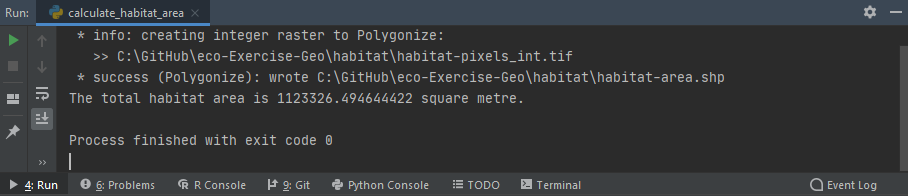
Figure 5:Successful run of the calculate_habitat_area.py script.
Plotted in QGIS, the habitat-area shapefile looks like this (use Categorized symbology):
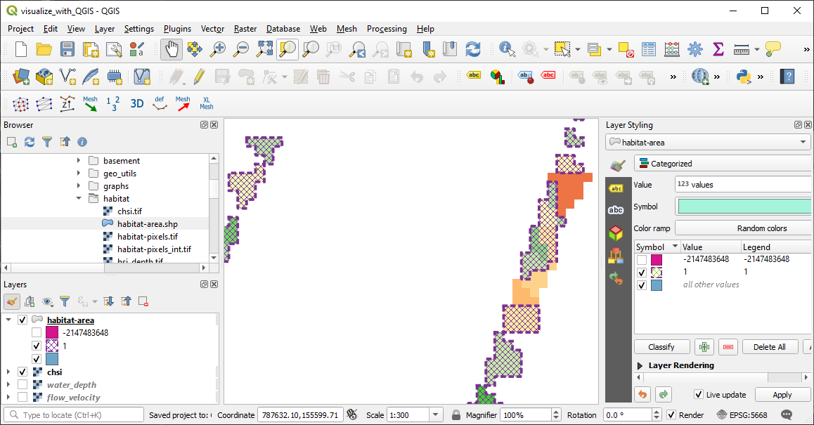
Figure 6:The habitat-area shapefile plotted in QGIS with Categorized symbology, where the usable habitat area ( 0.4) is delineated by the hatched purple patches and their dashed outlines.
Result Interpretation
The of the analyzed river section represents a very small share of the total wetted area, which can be interpreted as an ecologically poor status of the river. However, a glance at a map and the simulation files of the Flaz example of BASEMENT suggests that at a discharge of 50 m/s, a flood situation can be assumed. As during floods, there are generally higher flow velocities, which are out-of-favor of juvenile fish, the small usable habitat area is finally not surprising.
- Noack, M., Schneider, M., & Wieprecht, S. (2013). Ecohydraulics: an integrated approach (I. Maddock, A. Harby, P. Kemp, & P. Wood, Eds.; pp. 75–91). Wiley-Blackwell. 10.1002/9781118526576
- Bovee, K. D. (1986). Development and evaluation of Habitat Suitability Criteria for use in the instream flow incremental methodology (Techreport No. 21). National Ecology Center, U.S. Fish. https://pubs.er.usgs.gov/publication/70121265
- Stalnaker, C., Lamb, B. L., Henriksen, J., Bovee, K., & Bartholow, J. (1995). The Instream Flow Incremental Methodology - A Primer for IFIM. National Biological Service, U.S. Department of the Interior, Opler, Paul A. www.dtic.mil/cgi-bin/GetTRDoc?AD=ADA322762
- Yao, W., Bui, M. D., & Rutschmann, P. (2018). Development of eco-hydraulic model for assessing fish habitat and population status in freshwater ecosystems. Ecohydrology, 11(5), 1–17. 10.1002/eco.1961
- Tuhtan, J. A., Noack, M., & Wieprecht, S. (2012). Estimating stranding risk due to hydropeaking for juvenile European grayling considering river morphology. KSCE Journal of Civil Engineering, 16(2), 197–206. 10.1007/s12205-012-0002-5