When setting up the case folder, edits need to be done to the following files:
In the Constant folder: the various properties files and the boundary file in the polyMesh folder.
In the System folder: the setFieldsDict, fvSchemes, fvSolution and controlDict files.
In the 0 folder: all the containing files.
The Constant Subdirectory
After having copied the polyMesh folder from the snappyHexMesh results, it is necessary to correctly define the type of the different composing elements in the boundary file. For instance, in the example below, the Gravel-bottom element was defined as wall whereas the Inlet was defined as a patch.
FoamFile
{
    format      ascii;
    class       polyBoundaryMesh;
    location    "constant/polyMesh";
    object      boundary;
}
// * * * * * * * * * * * * * * * * * * * * * * * * * * * * * * * * * * * * * //

...

    Gravel-bottom
    {
        type            wall;
        inGroups        List<word> 1(wall);
        nFaces          132062;
        startFace       5105689;
    }
    Inlet
    {
        type            patch;
        inGroups        List<word> 1(wall);
        nFaces          288;
        startFace       5237751;
    }

 ...
Different patch types are available in OpenFOAM. For a detailed explanation refer to the boundaries section of the OpenFOAM User Guide.
patch: generic patch
symmetryPlane: plane of symmetry
empty: from and back planes of a 2D geometry
wedge: wedge front and back for an axi-symmetric geometry
cyclic: cyclic plane
wall: used to define wall functions in turbulent flow
processor: inter-processor boundary
The following files need to be added for defining the case properties along with a list of property files for the present case.
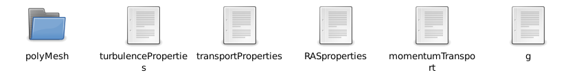
Figure 1:Contents of the constant folder.
In the turbulenceProperties files, the turbulence model is defined. OpenFOAM includes support for the following types of turbulence modeling:
Reynolds Averaged (Navier-Stokes) Simulation (RANS, referred to as RAS in OpenFOAM),
Detached Eddy Simulation (DES), and
Large Eddy Simulation (LES)
simulationType  RAS;

RAS
{
    RASModel        kEpsilon;

    turbulence      on;

    printCoeffs     on;
}
The transportProperties file defines the properties of the two phases considered in the present case (air and water) and the surface tension between the two phases.
phases (water air);

water
{
    transportModel  Newtonian;
    nu              [0 2 -1 0 0 0 0] 1e-06;
    rho             [1 -3 0 0 0 0 0] 1000;
    CrossPowerLawCoeffs
    {
        nu0             nu0 [ 0 2 -1 0 0 0 0 ] 1e-06;
        nuInf           nuInf [ 0 2 -1 0 0 0 0 ] 1e-06;
        m               m [ 0 0 1 0 0 0 0 ] 1;
        n               n [ 0 0 0 0 0 0 0 ] 0;
    }

    BirdCarreauCoeffs
    {
        nu0             nu0 [ 0 2 -1 0 0 0 0 ] 0.0142515;
        nuInf           nuInf [ 0 2 -1 0 0 0 0 ] 1e-06;
        k               k [ 0 0 1 0 0 0 0 ] 99.6;
        n               n [ 0 0 0 0 0 0 0 ] 0.1003;
    }
}

air
{
    transportModel  Newtonian;
    nu              [0 2 -1 0 0 0 0] 1.48e-05;
    rho             [1 -3 0 0 0 0 0] 1;
    CrossPowerLawCoeffs
    {
        nu0             nu0 [ 0 2 -1 0 0 0 0 ] 1e-06;
        nuInf           nuInf [ 0 2 -1 0 0 0 0 ] 1e-06;
        m               m [ 0 0 1 0 0 0 0 ] 1;
        n               n [ 0 0 0 0 0 0 0 ] 0;
    }

    BirdCarreauCoeffs
    {
        nu0             nu0 [ 0 2 -1 0 0 0 0 ] 0.0142515;
        nuInf           nuInf [ 0 2 -1 0 0 0 0 ] 1e-06;
        k               k [ 0 0 1 0 0 0 0 ] 99.6;
        n               n [ 0 0 0 0 0 0 0 ] 0.1003;
    }
}

sigma           [1 0 -2 0 0 0 0] 0.072;
When selecting the RAS turbulence model, also the RASproperties sub-dictionary must be added. This file contains the keywords defining the name of the RAS turbulence model, the option to either turn turbulence modeling on or off, and a switch to print the model coefficients to the terminal at the simulation startup.
RASModel        kEpsilon;
turbulence      on;
printCoeffs     on;
The momentumTransport dictionary is read by any solver that includes turbulence modeling. The keywords defined in this sub-dictionary are the same as the above-described ones.
simulationType  RAS;

RAS
{
    model           kEpsilon;
    turbulence      on;
    printCoeffs     on;
}
Turbulence models can be listed by running a solver with the -listMomentumTransportModels option:
user@user123:~/OpenFOAM-9/channel/$ interFoam -listMomentumTransportModelsFinally, the g sub-dictionary simply defines the gravitational acceleration and the used units.
dimensions      [ 0 1 -2 0 0 0 0 ];
value           ( 0 0 -9.8065 );
The System Directory
The System Folder contains the parameters associated with the solution procedure itself. The mandatory files for running the simulation are the controlDict in which the run control parameters are set and those for data output; notably, the fvSchemes where the discretization schemes used in the solution can be selected and the fvSolution in which the equation solvers, tolerances, and other algorithm controls are set. Additionally, the setFieldsDict is added, which enables the user to set values on a selected set of cells/patch-faces.
In the controlDict file, several control parameters can be set as, for instance, the start & end times, and time step dT of the simulation. In particular, when running a cold start simulation (i.e., a case in which the channel is initially dry), the time step should be set to adjustable enabling the adjustment of the time step according to maximum CFL condition in the transient simulation. Additionally, the maximum value of the CFL condition maxCo and the maximum value at the interface maxAlphaCo should be assigned.
application     interFoam;
startFrom       startTime;
startTime       0;
stopAt          endTime;
endTime         3600;
deltaT          0.1;
writeControl    adjustableRunTime;
writeInterval   1;
purgeWrite      0;
writeFormat     binary;
writePrecision  6;
writeCompression uncompressed;
timeFormat      general;
timePrecision   6;

runTimeModifiable yes;
adjustTimeStep  yes;

maxCo           1.0;
maxAlphaCo      1.0;
maxDeltaT       1.0;
The fvSchemes dictionary in the system directory sets the numerical schemes for the terms that appear in the application that is being run. For the time schemes ddtSchemes, apart from the first-order accurate Euler scheme, other options are available, such as the second-order Crank-Nicholson and backward schemes. The gradient schemes gradSchemes are then defined. The available schemes are the Gauss gradient scheme and the Least-squares gradient scheme. The interpolation scheme can be either cell-based linear (linear) or point-based linear (pointLinear) or least squares (leastSquares). The divergence scheme to be used can be defined with the divSchemes keyword. Detailed information regarding the available options and corresponding syntax can be found in the divergence schemes section of the OpenFOAM User Guide. For the laplacianSchemes, all options are based on the application of the Gauss theorem, requiring thus an interpolation scheme to transform the coefficients from cell values to the faces, and a surface-normal gradient scheme. The interpolationSchemes are required to transform cell-center quantities to face centers. Several interpolation schemes are available, from the ones based uniquely on the geometry to, for example, convection schemes that are a function of the local flow.
ddtSchemes
{    default         Euler;}

gradSchemes
{    default         Gauss linear;}

divSchemes
{
    div(rhoPhi,U)   Gauss linearUpwind grad(U);
    div(phi,alpha)  Gauss interfaceCompression vanLeer 1;
    div(phi,k)      Gauss upwind;
    div(phi,epsilon) Gauss upwind;
    div(((rho*nuEff)*dev2(T(grad(U))))) Gauss linear;
}

laplacianSchemes
{    default         Gauss linear corrected;}

interpolationSchemes
{    default         linear;}

snGradSchemes
{    default         corrected;}

wallDist
{    method meshWave;}
The fvSolution files contains a set of sub-dictionaries that are specific to the solver being run. Additionally, there is a set of standard sub-dictionaries, including the solvers, relaxationFactors, PISO and SIMPLE, which cover most of the ones used by the standard solvers. An example of the set of entries required for the interFoam solver can be found in this eBook’s case folder (Simulation folder). A detailed overview of all available options can be found in the OpenFOAM User Guide (Solution and Algorithm Control).
The setFieldsDict allows the user to assign a certain value to a selected set of cells/patch-faces. For the present tutorial this dictionary was used to assign an initial water level to the inlet of the model. Multiple options are available for selecting the cells of interest. In the example shown below, the boxToCell option was selected, which selects all cells whose cell center is located inside the given bounding box.
defaultFieldValues
(
    volScalarFieldValue alpha.water 0
);

regions    // Select based on surface
(
    boxToCell
    {
        box (-3.6 5.1 -2.5) (0.4 -4.0 1.2);
        fieldValues
        (
            volScalarFieldValue alpha.water 1
        );
    }
);
Alternatively, other sources can be used, such as fieldToCell, which selects all cells characterized by a field value within the selected range [min; max]. A very useful option when setting the initial water level is also the surfaceToCell source that selects the cells using a surface, based on an imported STL surface. In this case the dictionary would look like:
defaultFieldValues
(
    volScalarFieldValue alpha.water 0
);

regions    // Select based on surface
(
  surfaceToCell
      {
          file            "./constant/triSurface/water.stl";
          outsidePoints   ((x y z));
          includeCut      true;
          includeInside   true;
          includeOutside  false;
          nearDistance    -1;
          curvature       -100;
          fieldValues
          (
              volScalarFieldValue alpha.water 1
          );
      }
 );
The outsidePoints keyword defines the outside of the surface. IncludeCut, includeInside, and IncludeOutside are booleans that determine whether to include in the selection the cells cut by the surface, the cells inside the surface, and/or outside the surface, respectively. The nearDistance keyword is a scalar that determines which cells with the center near to the surface to include. Finally, curvature includes the cells close to a strong curvature on the surface.
A complete list of all available sources can be found in the OpenFOAM Wiki in the TopoSet section.
The 0 Directory
The 0 directory is the time directory containing the files describing the initial conditions of the simulation. Inside this directory, one text file for each field is required for the interFoam solver executable. In the present case, these files include: for the flow velocity, p-rgh for the dynamic pressure, nut for the turbulent viscosity, for the turbulent kinetic energy, for the rate of dissipation of turbulent kinetic energy, and alpha.water.orig for the initial phases. The complete set of the files used for this tutorial can be found in the case folder.
Variable Dictionaries
U field Dictionary
This dictionary defines the boundary conditions and initial set up for the vector field. For the internalField uniform initial conditions with a value of (0 0 0) were set. For all remaining walls and patches, the following were assigned:
Air patch : pressureInletOutletVelocity condition, which assigns a zero gradient condition to the flow out of the domain and a velocity based on the flux in the patch-normal direction to the flow into the domain.
Concrete-sides, Gravel-bottom and Obstacle patches: noSlip condition. The patch velocity is set to (0 0 0)
Inlet patch: a flowRateInletVelocity condition was chosen. This allows to define the volumetric or mass flow rate at the inlet patch.
Outlet patch: a zeroGradient boundary condition was set. The internal values are therefore extrapolated to the boundary face.
dimensions      [0 1 -1 0 0 0 0]; //kg m s K mol A cd
internalField   uniform (0 0 0);

boundaryField
{
     Air
        {
        	type            pressureInletOutletVelocity;
         	value           uniform (0 0 0);
        }

     Concrete-sides
        {
        	type            noSlip;
        }

     Gravel-bottom
        {
        	type            noSlip;
        }

     Inlet
        {
        	type            flowRateInletVelocity;
        	volumetricFlowRate constant 0.5;
	}

     Obstacle
        {
        	type            noSlip;
        }

     Outlet
        {
                type            zeroGradient;
        }
}
p-rgh field dictionary
This dictionary defines the boundary conditions and initial set up for the dimensional field p-rgh, expressed in Pa. The internalField was initialized with a 0 value in the entire domain. The remaining fields were set as follows:
Air patch: the totalPressure was assigned. This condition sets the static pressure at the patch based on the specification of the total pressure and it allows to adequately represent the atmospheric pressure.
All other patches: the condition used was a fixedFluxPressure boundary. This boundary condition is utilized as an alternative to zeroGradient, in the cases in which also the gravity and surface tension are present in the solution equations.
dimensions      [1 -1 -2 0 0 0 0];//kg m s K mol A cd
internalField   uniform 0;//initially atmospheric pressure in the entire domain

boundaryField
{
     Air
        {
        	type            totalPressure;
        	p0              uniform 0;
        }

     Concrete-sides
        {
        	type            fixedFluxPressure;
        	value           uniform 0;
        }

     Gravel-bottom
        {
        	type            fixedFluxPressure;
        	value           uniform 0;
        }

     Inlet
        {
        	type            fixedFluxPressure;
        	value           uniform 0;
	}

     Obstacle
        {
        	type            fixedFluxPressure;
        	value           uniform 0;
        }

     Outlet
        {
                type            fixedFluxPressure;
        	value           uniform 0;
        }
}
nut field Dictionary
This dictionary defines the boundary conditions and initial set up for the turbulent viscosity nut, expressed in m/s. The internalField was initialized with a 0 value in the entire domain. The remaining fields were set as shown below:
Air, Inlet and Outlet patch: the condition was set to calculated, meaning that no value is prescribed and that it is calculated from the here used RANS turbulence model and the values for (turbulent kinetic energy) and in this case.
All remaining walls: the nutkRoughWallFunction boundary condition was applied.
This boundary condition provides a wall constraint on the turbulent viscosity. This allows to account for the effects of roughness. The implementation of the different materials present in the model was done by defining the different roughness heights ks (e.g., 0.0052 for the concrete walls).
dimensions      [0 2 -1 0 0 0 0];
internalField   uniform 0;

boundaryField
{

    Air
    {
      type            calculated;
      value           uniform 0;
    }

    Concrete-sides
    {
      type            nutkRoughWallFunction;
      Ks              uniform 0.0052;
      Cs              uniform 0.5;
      value           uniform 0;
    }

    Gravel-bottom
    {
      type            nutkRoughWallFunction;
      Ks              uniform 0.15;
      Cs              uniform 0.5;
      value           uniform 0;
    }

    Inlet
    {
      type            calculated;
      value           uniform 0;
    }

    Obstacle
    {
      type            nutkRoughWallFunction;
      Ks              uniform 0.0052;
      Cs              uniform 0.5;
      value           uniform 0;
    }

    Outlet
    {
        type            calculated;
        value           uniform 0;
    }
}
k field Dictionary
This dictionary defines the boundary conditions and initial setup for the turbulent kinetic energy , expressed in m/s. The internalField was initialized with a uniform value in the entire domain. The remaining fields were set as follows:
Air and Outlet patch: inletOutlet, which corresponds to a zeroGradient condition, with the exception of the case in which the velocity vector next to the boundary is directed inside the domain. In the latter case, it switches to a fixedValue condition.
Inlet patch: fixedValue. The corresponding value was the one assigned to the internalField.
All remaining walls: kqRWallFunction. This boundary condition provides a simple wrapper around the zero-gradient condition.
dimensions      [0 2 -2 0 0 0 0];
internalField   uniform 1.22e-03;

boundaryField
{
    Air
  {
      type            inletOutlet;
      inletValue      $internalField;
      value           $internalField;
  }

  Concrete-sides
  {
    type            kqRWallFunction;
    value           $internalField;
  }

  Gravel-bottom
  {
    type            kqRWallFunction;
    value           $internalField;
  }

  Inlet
  {
    type            fixedValue;
    intensity       0.05;
    value           $internalField;
  }

  Obstacle
  {
    type            kqRWallFunction;
    value           $internalField;
  }

  Outlet
  {
      type            inletOutlet;
      inletValue      $internalField;
      value           $internalField;
  }
}
epsilon field Dictionary
This dictionary defines the boundary conditions and initial set up for the rate of dissipation of turbulent kinetic energy, expressed in ms. The internalField was initialized with a uniform value in the entire domain. The remaining fields were set as shown below:
Air and Outlet patch: inletOutlet, as described above for .
Inlet patch: fixedValue, corresponding to the internalField value.
All remaining walls: epsilonWallFunction. This boundary condition provides a wall constraint on the turbulent kinetic energy dissipation rate and the turbulent kinetic energy production contribution for low and high Reynolds number turbulence models.
dimensions      [0 2 -3 0 0 0 0];
internalField   uniform 3.20e-05;

boundaryField
{
    Air
    {
        type            inletOutlet;
        inletValue      $internalField;
        value           $internalField;
    }

    Concrete-sides
    {
      type            epsilonWallFunction;
      value           $internalField;
    }

    Gravel-bottom
    {
      type            epsilonWallFunction;
      value           $internalField;
    }

    Inlet
    {
      type            fixedValue;
      value           $internalField;
    }

    Obstacle
    {
      type            epsilonWallFunction;
      value           $internalField;
    }

    Outlet
    {
        type            inletOutlet;
        inletValue      $internalField;
        value           $internalField;
    }
}
alpha.water field Dictionary
This dictionary defines the boundary conditions and initial conditions for the non-dimensional field alpha.water. The internalField was initialized with a uniform value equal to 0 in the entire domain, meaning no water is present in the domain at time 0. The water will then be initialized running the setFields command with the settings defined in the corresponding dictionary. The remaining fields were set as shown below:
Air patch: inletOutlet, which avoids the possibility of water flowing back into the domain. In the case in which the flow is exiting, a zeroGradient condition is applied, and similarly, if the flow is returning a value equal to the one defined as inletValue.
Inlet patch: fixedValue, corresponding to a uniform value of 1, meaning the entire patch is only composed by water (no air phase present).
Outlet patch and all remaining walls: zeroGradient. In this case, the internal values are extrapolated to the boundary face.
dimensions      [0 0 0 0 0 0 0];

internalField   uniform 0;

boundaryField
{
  Air
  {
    type            inletOutlet;
    inletValue      uniform 0;
    value           uniform 0;
  }

  Concrete-sides
  {
    type            zeroGradient;
  }

  Gravel-bottom
  {
    type            zeroGradient;
  }

  Inlet
    {
        type            fixedValue;
        value           uniform 1;
    }

  Obstacle
  {
    type            zeroGradient;
  }

    Outlet
  {
    type            zeroGradient;
  }
}