Support Vector Machines (SVM)
This tutorial features the Support Vector Machine (SVM) technique for classifying riverbed morphology types as a function of hydraulic and sediment transport data. This notebook represents an extended Python exercise for a supervised learning application with a non-linear model.
Enable interactive reading and executing code blocks with  and find morphology-predictor-svm.ipynb. Alternatively, install Python and JupyterLab locally and download this Jupyter notebook.
Theory
In the field of restoration science, the identification of river morphology provides essential insights, for instance, to guide targeted terraforming aiming at re-instating a near-natural state of a fluvial landscape. In addition, morphological patterns may serve as predictors for estimating fluvial sediment transport and vice versa. Thus, there is a bidirectional relationship between fluvial hydraulics, sediment transport, and morphological patterns, which represent physical habitat for aquatic species and may even affect energy production Recking et al., 2016.
Yet, classifying and predicting fluvial morphodynamics is challenging because of the complexity of river ecosystems and every river being a unique environment. However, there are repeating morphological units of rivers with similar characteristics. A basic set of repetitive morphological features was introduced by Montgomery & Buffington (1997), and we will focus in this tutorial on the following five morphological units (click on the items to read more):
Roughly, these morphological units follow the above-listed order along a river with decreasing channel slope, from the steep headwaters toward the estuary, though local controls (e.g., sediment supply, confinement, or tributaries) may interrupt this sequence. Thus, step pool units can typically be found in steep upstream (mountain) river sections, while sand beds predominantly occur in low-gradient lowland river sections, close to estuaries or confluences. Note that there are many other morphological units besides, such as slackwater, swales, or bars Wyrick & Pasternack, 2014. Figure 1 illustrates some morphological units of near-natural rivers.
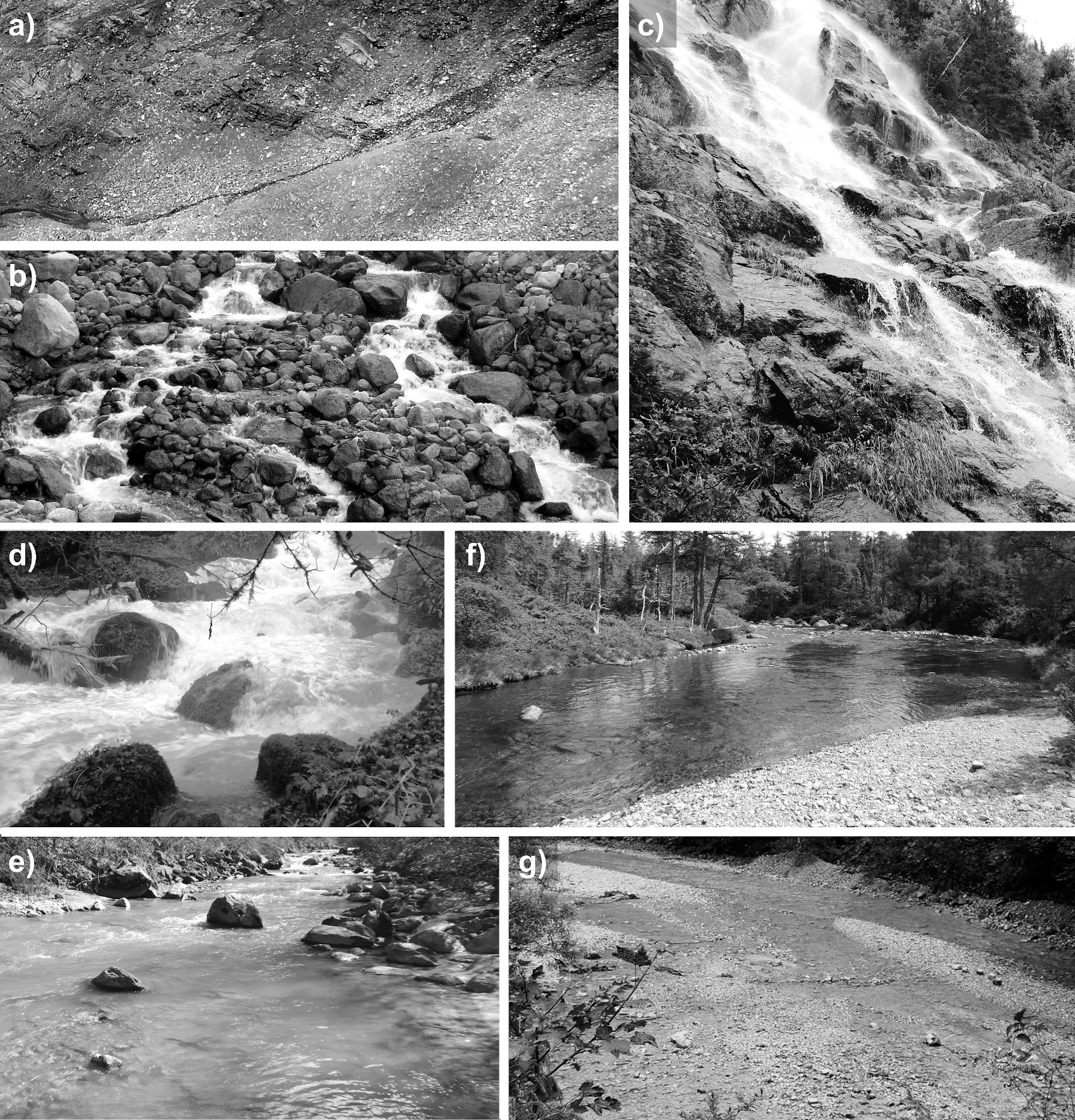
Figure 1:a) A colluvial headwater stream (Furtschaglbach, Austria), b) a cascade stream (Torrent des Favrands, France), c) a bedrock stream (Anse St-Jean, Québec, Canada), d) a step-pool stream (Dessoubre, France), e) a plane-bed stream (Dranse, Switzerland), f) a riffle-pool stream (Le diable, Québec, Canada), g) a braided stream (Jenbach, Germany). Source: Schwindt (2017)
To guide restoration actions, experts often visually classify morphological units on-site, though some of them may also be distinguishable on aerial imagery. On-site (in-situ) expert assessments may also serve as ground truth for machine learning models. In this exercise, we will use hydrodynamic parameters with expert-based ground truth from the database https://
Pre-processing
Load Data
We downloaded a dataset from https://
The samples stem from cross-sections of 146 different rivers around the globe.
The dataset embraces hydraulic and sediment transport parameters (e.g., grain sizes), though in this tutorial, we will only use the following parameters to train the SVM model:
W: Channel width (m)
S: Channel slope (m/m)
Q: Discharge (m s)
U: Bulk flow velocity (m s)
H: Water depth (m)
In a machine learning context, these parameters for predicting morphological units are also called features. The first step is to load (and view) the data as a pandas.DataFrame:
import pandas as pd

data = pd.read_csv("data/bedload_dataset")
dataClean the Dataset
To avoid the SVM model being affected by statistics based on nonsense entries (e.g., Not-a-Number NaN values) or extreme outliers, for instance, resulting from typos, we will apply some cleaning methods.
Remove NaN Values
The first cleaning step is to remove NaNs that may later lead the SVM model to bad conclusions.
# dataset essential info
data.info()
print()

# remove rows that contain at least one NaN value
data.dropna(inplace=True)

# verify that all NaN values were removed
for column in data.columns.to_list():
    print(column, ":", data[column].isnull().any())

# verify final shape of the dataset
print(data.shape)
<class 'pandas.DataFrame'>
RangeIndex: 1067 entries, 0 to 1066
Data columns (total 6 columns):
# Column Non-Null Count Dtype
--- ------ -------------- -----
0 W 1067 non-null float64
1 S 1067 non-null float64
2 Q 1067 non-null float64
3 U 1067 non-null float64
4 H 1067 non-null float64
5 Morphology 1067 non-null str
dtypes: float64(5), str(1)
memory usage: 59.7 KB
W : False
S : False
Q : False
U : False
H : False
Morphology : False
(1067, 6)
Search Outliers
Outliers may occur in extreme environments or under extreme conditions (e.g., intense precipitation), but some of them also stem from equipment failures that will affect the performance of the SVM model. Thus, recognizing and removing such device-related outliers is an essential step.
Visualizing the features in scatter plots can be helpful to spot outlier candidates. The following code block creates a scatter plot of every feature, and marks its mean value (horizontal line) and the range of ±2 standard deviations around it (vertical line, assuming a Gaussian-like distribution).
import numpy as np
import matplotlib.pyplot as plt

# plot visualization parameters
labels = data.columns[0:5].tolist()
colors = ["crimson", "purple", "limegreen", "gold", "blue"]
width = 0.5
rng = np.random.default_rng(42)  # seed for a reproducible horizontal jitter

# one subplot per feature because the features have different units and magnitudes
fig, axes = plt.subplots(1, len(labels), figsize=(12, 4))
for ax, label, color in zip(axes, labels, colors):
    x = rng.random(data.shape[0]) * width - width / 2.
    ax.scatter(x, data[label], color=color, s=8)
    mean = data[label].mean()
    std = data[label].std()
    ax.plot([-width / 2., width / 2.], [mean, mean], color="k")
    ax.plot([0, 0], [mean - 2 * std, mean + 2 * std], color="k")
    ax.set_xticks([])
    ax.set_xlabel(label)

fig.tight_layout()
plt.show()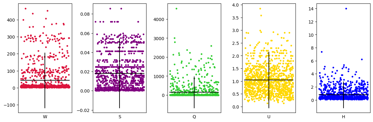
Remove Outliers
Outliers can be removed with two different methods:
Manual (i.e., expert judgment): identify outliers of the features and remove them by setting limits of their interval.
Automated: assume a probability distribution and set limits based on a low probability of occurrence.
The following code block implements these two (manual-expert and automated) methods. The manual outlier removal is hard-coded because the limits should be given by experts.
The automated approach (below the else statement) assumes that the data follow a Gaussian distribution, and removes data points with a so-called z-score of more than 4 (four) in absolute terms. The z-score expresses by how many standard deviations a value deviates from the mean. For a Gaussian distribution, approximately 99.994 % of all values lie within four standard deviations from the mean. Thus, a sample with an occurrence probability of less than 0.01 % is automatically considered an outlier and removed from the dataset. To this end, we use the zscore function of the scipy library.
from scipy.stats import zscore
# choose the method to remove outliers
# remove_method = "expert_analysis"
remove_method = "zscore"

if "expert" in remove_method:
    data = data.loc[(data["Q"] < 2000) &
                    (data["W"] < 250)]
else:
    data = data[(np.abs(zscore(data.loc[:, data.columns != "Morphology"])) < 4).all(axis=1)]

# work on an independent copy of the filtered rows (avoids chained assignment issues)
data = data.copy()
dataVerify Class Proportions
A machine learning model requires the ground truth data to comply with some quality standards. Those involve (among others):
Every model needs a different minimum number of samples to have statistical significance. It is not a trivial task to identify the minimum number of samples that yield a trustworthy model. However, to represent a class properly (whatever that means), the so-called frequency distribution of every feature must be similar to the population frequency distribution.
Having more than 30 samples when dealing with normally distributed variables is a good-practice rule of thumb.
Ideally, the classes used for a classification problem should be represented by a similar number of samples. An unbalanced dataset may produce a model that gives preference to correctly classifying the class with a larger number of samples. This is a consequence of using accuracy as a performance metric. Accuracy is the ratio of correct predictions and the total number of predictions (). By favoring the total number of correct predictions over a balanced one, accuracy masks the importance of correctly predicting the under-represented classes. Therefore, class-sensitive metrics, such as precision and recall, are preferable for measuring the performance of models trained on unbalanced data.
Solutions for balancing unbalanced samples embrace:
Collecting new data or generating synthetic data (e.g., by oversampling the under-represented classes or with Monte Carlo methods).
Weighting classes, which means to assign higher weights to under-represented classes to increase their importance in the training process. The effect of weights or decision thresholds on the trade-off between true and false positive rates can be evaluated with an ROC curve.
In this tutorial, the samples can be considered balanced, except for the sand bed class (see output below). Weighting and ROC curves are not considered here. If the sensitivity and specificity of the sand bed class were acceptable when classifying test data, the model could also be used for sand bed classification without the need for balancing techniques.
data["Morphology"].value_counts()Morphology
Step-pool 247
Plane Bed 243
Riffle-pool 241
Braiding 228
Sand bed 79
Name: count, dtype: int64Derive New Predictors
Sometimes it is possible to compute new meaningful features from the existing ones. For instance, known predictors for morphology are:
the product of (energy) slope (-), bulk flow velocity (m/s), and water depth (m), which is proportional to the specific stream power (W/m), where is the density of water and is gravitational acceleration; similarly, the product of and is proportional to the bed shear stress
the ratio of discharge (m/s) and width (m), which is the unit discharge (m/s)
# compute new columns for the new features SUH and Q/W
data["SUH"] = data["S"] * data["U"] * data["H"]
data["Q/W"] = data["Q"] / data["W"]
dataVerify Multicollinearity
Correlated features (i.e., statistically dependent measurement parameters) may result in unreliable models. For instance, consider a scientist who wants to use machine learning (ML) models to predict the number of tourists that get sunburned in Brazil during their vacation. She wants to use solar radiation intensity and the number of ice cream scoops sold as features. The scientist may find that both features are relevant to predict the number of sunburned tourists, but the reason for this finding is that the number of ice cream scoops sold and solar radiation intensity are correlated. Thus, the scientist has no way to know the real importance of each feature in predicting sunburned tourists because the features grow and decrease simultaneously. By the way, ice cream consumption does not cause sunburns (nor vice versa); both are driven by a common cause (sunshine), but that is another subject.
To this end, it is important to investigate the correlation among features and consider eliminating correlated features to produce a more reliable model. One way to visually spot collinearity is plotting the combination of two variables in a scatter plot. For this purpose, the below figure aids in spotting the following aspects of the bedload_dataset:
There is a strong linear correlation between the and features, which is not surprising because .
There is only a weak linear correlation between and (correlation coefficient of approximately 0.37, see the heatmap below).
The flow velocity distribution is roughly bell-shaped (see main diagonal).
import seaborn as sns

# plot scatter of the 2d (two-dimensional) combination of features
sns.pairplot(data.loc[:, data.columns != "Morphology"])
plt.show()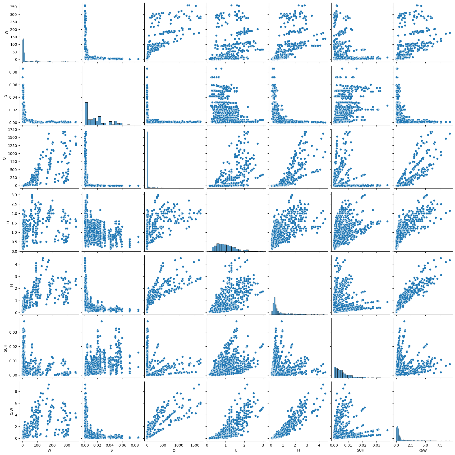
In addition, a heatmap is another efficient method to visualize linear correlation among features. Also computing linear correlation enables quantitative analysis.
# verify linear correlation
feature_corr_df = data.loc[:, data.columns != "Morphology"].corr()
mask = np.zeros_like(feature_corr_df, dtype=bool)
mask[np.triu_indices_from(mask)] = True
sns.heatmap(feature_corr_df,
            annot=True,  # print value inside the grid
            mask=mask  # mask values (boolean matrix)
            )
plt.show()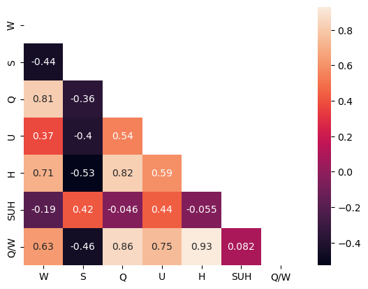
Variance Inflation Factor (VIF)
A straightforward method to evaluate multicollinearity is computing the Variance Inflation Factor (VIF) for every feature, which quantifies how well a feature can be explained by the other features.
The first step to compute the VIF is treating a feature as a dependent variable and fitting a linear regression model using the other features as independent variables. Second, store the corresponding coefficient of determination yielded by the linear model.
Finally, the VIF can be computed for each feature with the following equation:
is the variance inflation factor of the -th feature, and
is the coefficient of determination resulting from the linear regression of the -th feature on all other features.
Note that the larger (i.e., the better the linear regression model), the greater is the inflation. In other words, large VIF values indicate a high correlation of the feature under consideration with at least one of the other features. Still, it is not possible to say based on the VIF only, which other feature is causing the VIF to inflate.
As a rule of thumb, a VIF greater than 10 (ten) indicates an unsuitable set of features to produce a reliable ML model. Ideally, the VIF should remain smaller than 5 (five), which is considered moderate correlation Franke, 2010. However, these reference values are not a generally and always applicable rule. A VIF equal to or greater than 10 can still yield a good model.
Further analysis to study the impact of a high VIF on correlated features can be carried out by removing one feature at a time and investigating how the feature removal affects the variation of the standard error and p-value of the model.
In this tutorial, 2 features have a VIF 10 (notably, and ), as the following code block shows.
from sklearn.linear_model import LinearRegression

# compute VIF for the features
def calculate_vif(df, features):
    vif = {}

    for feature in features:
        # extract all the other features you will regress against
        X = [f for f in features if f != feature]
        X, y = df[X], df[feature]

        # extract r-squared from the fit
        r2 = LinearRegression().fit(X, y).score(X, y)

        # compute VIF
        vif[feature] = 1 / (1 - r2)
    # return VIF DataFrame
    return pd.DataFrame({"VIF": vif})

# call function calculate_vif with features as input
calculate_vif(df=data,
features=data.columns[data.columns != "Morphology"].to_list())Remove Features to Reduce VIF
With the goal of reducing the feature VIFs to less than 5, we use a trial-and-error approach in this tutorial. Modifying the below code block shows that removing and is enough to reduce the VIFs of the remaining features to less than 5. In particular, these two removed variables also go into the above-introduced features and . Thus, although and are removed, they still “contribute information” to the final model.
Combining correlated features to produce a new one, and later removing them, is a common approach to reduce VIFs. Since we yielded good VIF values by removing some of the features, no further analysis is necessary.
Finally, the features that are used to train and test the SVM model are shown by the output of the code block below.
# trial-and-error approach: remove features to get VIFs < 5
data = data.loc[:, (data.columns != "H") & (data.columns != "Q")]

# compute VIF again to verify if VIFs are less than 5
calculate_vif(df=data,
features=data.columns[data.columns != "Morphology"].to_list())Split Test and Training Datasets
The last preparation step for building the SVM model is to derive a training and a testing dataset from the entire bedload_dataset. Choosing a share of the data to compose a training and a testing dataset is commonly a heuristic choice. Here, we use 30 % of the data for testing a final hypothesis later. Note that inside the split datasets, the indices of the samples (rows of the tabular data) correspond to the indices of their classes in the target datasets.
from sklearn.model_selection import train_test_split


# split dataframes with features and labels only
labels = data.loc[:, "Morphology"]
predictors = data.loc[:, data.columns[data.columns != "Morphology"]]

# split testing set as 30% of the data
# X corresponds to the features (matrix form)
# y corresponds to the labels (vector form)
X_train, X_test, y_train, y_test = train_test_split(predictors,
                                                    labels,
                                                    test_size=0.3,
                                                    random_state=42  # seed for random selection of data
                                                    )

# visualize training and testing sets
print("TRAINING DATASET PREDICTORS")
print(X_train.head(), "\n")
print("dataframe size", X_train.shape, "\n")
print("------------------------------------------")
print("TRAINING DATASET TARGET")
print(y_train, "\n")
print()
print("------------------------------------------------------------------------------------\n")

print("TESTING DATASET PREDICTORS")
print(X_test.head())
print("dataframe size", X_test.shape, "\n")
print("------------------------------------------")
print("TESTING DATASET TARGET")
print(y_test.head())
print("Vector size", y_test.shape)
TRAINING DATASET PREDICTORS
W S U SUH Q/W
256 6.91 0.01100 1.02 0.003366 0.277858
397 88.09 0.00210 1.99 0.008149 3.889545
586 14.02 0.02070 1.34 0.022190 1.078459
526 218.00 0.00041 0.52 0.000175 0.541284
9 8.00 0.02000 1.18 0.007316 0.370000
dataframe size (726, 5)
------------------------------------------
TRAINING DATASET TARGET
256 Plane Bed
397 Plane Bed
586 Step-pool
526 Sand bed
9 Riffle-pool
...
89 Riffle-pool
337 Plane Bed
476 Plane Bed
123 Riffle-pool
876 Braiding
Name: Morphology, Length: 726, dtype: str
------------------------------------------------------------------------------------
TESTING DATASET PREDICTORS
W S U SUH Q/W
203 2.57 0.01040 1.58 0.008216 0.793774
937 105.00 0.00096 1.90 0.002918 3.076190
546 93.00 0.00050 1.10 0.001320 2.688172
214 53.04 0.00380 1.44 0.004596 1.211916
312 6.28 0.02020 0.34 0.001511 0.074841
dataframe size (312, 5)
------------------------------------------
TESTING DATASET TARGET
203 Riffle-pool
937 Braiding
546 Sand bed
214 Riffle-pool
312 Plane Bed
Name: Morphology, dtype: str
Vector size (312,)
Build the SVM Model
Working Principle
A Support Vector Machine (SVM) is a learning algorithm that searches for a so-called hyperplane that optimally separates feature classes. To find an optimal separation, the algorithm tries to maximize the distance (or margin) from the hyperplane to the nearest data points. The data points located on (or inside) the limits of the margin are also denominated support vectors because they work as a reference to draw the hyperplane (see Figure 2 below).
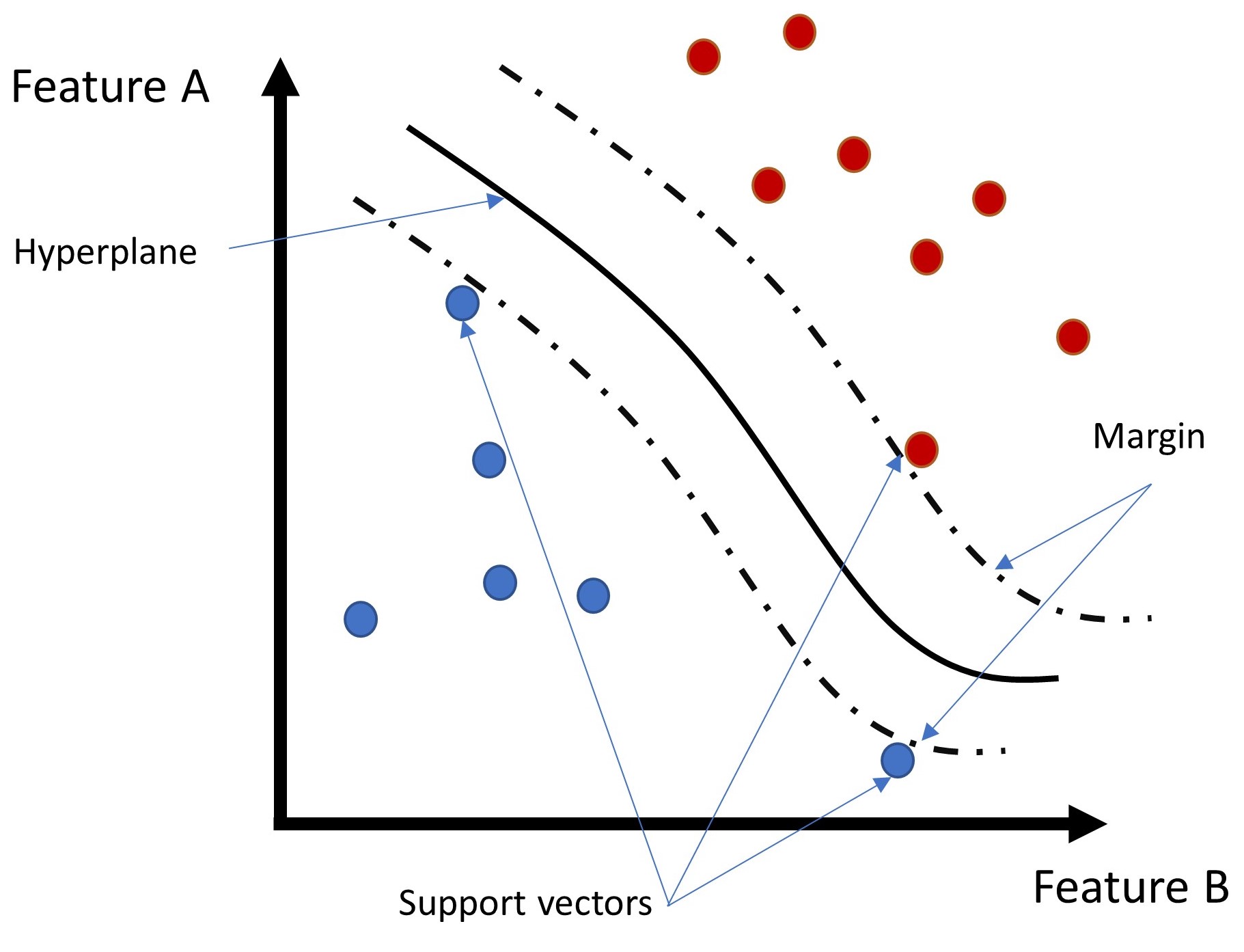
Figure 2:Illustration of a hyperplane and margins of an SVM. Source: Ricardo Barros
For instance, assume that two of the above classes are linearly separable. The separating hyperplane is defined by , and the regions that contain each class can be defined as:
--> Class Red, and --> Class Blue
where
is the vector of weights (normal to the hyperplane),
is the feature vector of a sample,
is the intercept (also called bias), and
the value of 1 is a scaling convention, since and can be multiplied by any positive factor without changing the hyperplane.
With this convention, the margin width is . Thus, maximizing the margin (after some steps that are not discussed here) corresponds to minimizing the following expression:
where is the transposed weight vector, subject to the constraint that all training samples lie on the correct side of the margin.
In the real world, however, it is common to find problems where classes are not linearly separable. In such situations, so-called kernels can be applied. A kernel is a function that implicitly maps the features into a space with higher dimensions (i.e., new features that are combinations of the available features), where the classes may become linearly separable. The so-called kernel trick makes this possible without explicitly computing the new features.
Here, we apply the Radial Basis Function (RBF) kernel. The RBF is a popular kernel because it implicitly maps into an infinite-dimensional feature space, which makes it very flexible. However, this flexibility also means that an RBF-SVM can overfit the training data when its parameters are not carefully tuned (see the next section).
k-Fold Cross Validation
SVMs with an RBF kernel can be tuned with two parameters:
C: determines how permissive the margins are. It differentiates between a hard margin (i.e., a margin that enables little or no penetration of data points) and a soft margin (i.e., a margin that enables penetration of data points inside the margin). A higher C corresponds to a harder margin.
gamma: determines the region of similarity among samples. It is the only parameter of the RBF kernel. The higher gamma is, the narrower is the influence of a labeled sample on classifying a new sample (i.e., only very close samples are considered similar).
Hard margins can also be interpreted as the sensitivity of the hyperplane when fitting it to the data. The harder the margin, the more the hyperplane twists to not allow any data point to penetrate the margin. Thus, both a high C and a high gamma increase the risk of overfitting.
In this tutorial, we define C based on a trial-and-error approach and gamma based on a five-fold cross-validation. The following code block builds the SVM using the sklearn library, and plots the validation and training error curves resulting from varying gamma.
from sklearn.svm import SVC
from sklearn.model_selection import validation_curve


# define C, gamma range, kernel and number of cross-val. folds
param_range = np.logspace(-5, 3, 13)  # gamma values to test
C = 500  # chosen hyperparameter through tuning
kernel = "rbf"  # radial basis function
n_of_folds = 5

# perform 5-fold cross-validation and save training and validation error
train_scores, test_scores = validation_curve(SVC(kernel=kernel,
                                                 C=C),
                                             X_train,
                                             y_train,
                                             param_name="gamma",
                                             param_range=param_range,
                                             scoring="accuracy",
                                             cv=n_of_folds
                                             )

# convert accuracy into error
train_error = 1 - train_scores
validation_error = 1 - test_scores

# compute 5-fold cross-validation mean and std of error
train_error_mean = np.mean(train_error, axis=1)
train_error_std = np.std(train_error, axis=1)
validation_error_mean = np.mean(validation_error, axis=1)
validation_error_std = np.std(validation_error, axis=1)

#-------------------------------------------------------------------

# visualization of training and error validation
plt.title("Validation Curve with SVM")
plt.xlabel(r"$\gamma$")
plt.ylabel("Error (1-accuracy)")
plt.ylim(-0.01, 1.1)
lw = 2
plt.semilogx(
    param_range, train_error_mean, label="Training error", color="darkorange", lw=lw
)
plt.fill_between(
    param_range,
    train_error_mean - train_error_std,
    train_error_mean + train_error_std,
    alpha=0.2,
    color="darkorange",
    lw=lw,
)
plt.semilogx(
    param_range, validation_error_mean, label="Cross-validation error", color="navy", lw=lw
)
plt.fill_between(
    param_range,
    validation_error_mean - validation_error_std,
    validation_error_mean + validation_error_std,
    alpha=0.2,
    color="navy",
    lw=lw,
)
plt.legend(loc="best")
plt.show()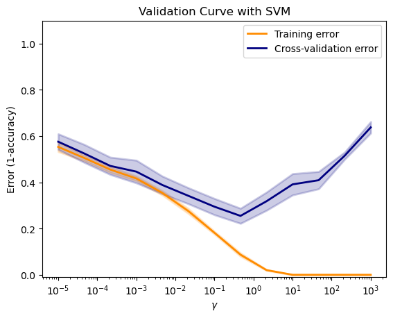
Select Optimum Parameters
The decision on optimum parameters for the SVM depends on your judgment. For the purpose of selecting optimum parameters in this tutorial, the below code block quantifies the above-shown plot (in particular, the blue curve) in tabular form and saves the gamma that yields the smallest error (gamma_opt).
# save optimal gamma
index_min = int(np.argmin(validation_error_mean))
validation_error_min = validation_error_mean[index_min]
gamma_opt = param_range[index_min]  # gamma that gives minimum validation error

# visualize error evolution with gamma
columns = ["Mean validation error", "gamma"]
array = np.array([validation_error_mean, param_range]).transpose()

print(pd.DataFrame(array, columns=columns), "\n")
print("Minimum mean validation error:", validation_error_min)
print("optimal gamma:", gamma_opt)
Mean validation error gamma
0 0.575739 0.000010
1 0.524856 0.000046
2 0.471101 0.000215
3 0.446311 0.001000
4 0.388474 0.004642
5 0.341606 0.021544
6 0.294709 0.100000
7 0.254861 0.464159
8 0.318262 2.154435
9 0.391252 10.000000
10 0.409173 46.415888
11 0.515144 215.443469
12 0.637789 1000.000000
Minimum mean validation error: 0.2548606518658479
optimal gamma: 0.46415888336127725
Train Optimum Hypothesis SVM Model
After defining a gamma yielding the smallest validation error (gamma_opt), we can train an optimal hypothesis (h_opt) model on the entire training dataset. In addition, we can evaluate the accuracy of the model by using it to classify the testing dataset. The below code block features the training procedure, fitting of the SVM (i.e., an optimum hypothesis), and prints the error of the optimum hypothesis on the testing dataset.
# train optimal model and evaluate accuracy
h_opt = SVC(kernel=kernel,
            gamma=gamma_opt,
            C=C)  # instantiate optimal model
h_opt.fit(X_train, y_train)  # train the model with entire training set
print("Error (1-Accuracy) of h_opt on testing data: \n -->>", 1 - h_opt.score(X_test, y_test))
Error (1-Accuracy) of h_opt on testing data:
-->> 0.19551282051282048
Performance Evaluation (Confusion Matrix)
Finally, the following code block generates the so-called confusion matrix to evaluate the optimum hypothesis model performance when classifying the samples with distinct morphologies. The confusion matrix uses the total number of samples and visualizes their true and predicted morphological units.
from sklearn.metrics import ConfusionMatrixDisplay

# plot confusion matrix
ConfusionMatrixDisplay.from_estimator(h_opt,  # trained optimal hypothesis model
                                      X_test,
                                      y_test,
                                      )
plt.xticks(rotation=45)
plt.show()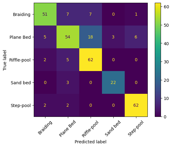
The confusion matrix of an exact model only has diagonal entries larger than zero, while all others are zero. The above-shown confusion matrix shows that our SVM model performs well in predicting step-pool (62 out of 66 true-label observations) and riffle-pool (62 out of 69) morphologies. Despite the smaller number of observations, the model also predicts most sand bed observations correctly (22 out of 25). However, these 25 true-label sand bed observations (opposed to 66 step-pool or 86 plane bed observations) are few, which makes the sand bed statistics less robust. Thus, the sand bed observations are unbalanced, and a solution for increasing the reliability could be to sample more sand bed morphological units (as explained above).
The weakest performance concerns plane bed morphologies: only 54 out of 86 true-label plane bed observations were predicted correctly. In particular, the model predicted 18 times riffle-pool and 6 times step-pool, where in reality (true label), plane bed morphological units prevailed. In addition, the model wrongly predicted one braiding observation to be a step-pool observation. These confusions are plausible from a physical point of view because plane beds represent a transitional morphology between step-pool and riffle-pool channels Montgomery & Buffington, 1997.
- Montgomery, D. R., & Buffington, J. (1997). Channel-reach morphology in mountain drainage basins. Geological Society of America Bulletin, 109(5), 596–611. https://doi.org/10.1130/0016-7606(1997)109<;0596:CRMIMD>2.3.CO;2
- Recking, A., Piton, G., Vazquez-Tarrio, D., & Parker, G. (2016). Quantifying the morphological print of bedload transport. Earth Surface Processes and Landforms, 41(6), 809–822.
- Wyrick, J. R., & Pasternack, G. B. (2014). Geospatial organization of fluvial landforms in a gravel-cobble river: Beyond the riffle-pool couplet. Geomorphology, 213(Supplement C), 48–65. 10.1016/j.geomorph.2013.12.040
- Schwindt, S. (2017). Hydro-morphological processes through permeable sediment traps [Thesis No. 7655, Laboratory of Hydraulic Constructions (LCH), Ecole Polytechnique fédérale de Lausanne (EPFL)]. 10.5075/epfl-thesis-7655
- Franke, G. R. (2010). Multicollinearity. Wiley International Encyclopedia of Marketing.