Get ready by cloning the exercise repository:
git clone https://github.com/Ecohydraulics/Exercise-SequentPeak.git
Figure 1:New Bullards Bar Dam in California, USA (source: Sebastian Schwindt 2017).
Theory
Seasonal storage reservoirs retain water during wet months (e.g., monsoon, or rainy winters in Mediterranean climates) to ensure sufficient drinking water and agricultural supply during dry months. For this purpose, enormous storage volumes are necessary, which often exceed 1,000,000 m.
The necessary storage volume is determined from historical inflow measurements and target discharge volumes (e.g., agriculture, drinking water, hydropower, or ecological residual water quantities). The sequent peak algorithm Potter, 1977 based on Rippl (1883) is a decades-old procedure for determining the necessary seasonal storage volume based on a storage volume curve (SD curve). The below figure shows an exemplary curve with volume peaks (local maxima) approximately every 6 months and local volume minima between the peaks. The volume between the last local maximum and the lowest following local minimum determines the required storage volume (see the bright-blue line in the figure).

Figure 2:Scheme of the sequent peak algorithm.
The sequent peak algorithm repeats this calculation over multiple years and the highest volume observed determines the required volume.
In this exercise, we use daily flow measurements from Vanilla River (in Vanilla-arid country with monsoon periods) and target outflow volumes to supply farmers and the population of Vanilla-arid country with sufficient water during the dry seasons. This exercise guides you through loading the daily discharge data, creating the monthly (storage) curve, and calculating the required storage volume.
Pre-processing of Flow Data
The daily flow data of the Vanilla River are available from 1979 through 2001 in the form of .csv files (flows folder).
Write a Function to Read Flow Data
The function will loop over the csv file names and append the file contents to a dictionary of numpy arrays. Make sure to import numpy as np, import os, and import glob.
Choose a function name (e.g.,
def read_data(args):) and use the following input arguments:directory: string of a path to filesfn_prefix: string of file prefix to strip dict-keys from a file namefn_suffix: string of file suffix to strip dict-keys from a file nameftype: string of file endingsdelimiter: string of column separator
In the function, test if the provided directory ends on
"/"or"\\"with
directory.endswith("/") or directory.endswith("\\")
and read all files that end withftype(we will useftype="csv"here) with thegloblibrary:if True:get the the csv (ftype) file list as
file_list = glob.glob(directory + "*." + ftype.strip(".").if False:get the the csv (ftype) file list as
file_list = glob.glob(directory + "/*." + ftype.strip(".")(the difference is only one powerful"/"sign).
Create the void dictionary that will contain the file contents as numpy arrays:
file_content_dict = {}Loop over all files in the file list with
for file in file_list:Generate a key for
file_content_dict:Detach the file name from the
file(directory + file name + file endingftype) withraw_file_name = file.split("/")[-1].split("\\")[-1].split(".csv")[0]Strip the user-defined
fn_prefixandfn_suffixstrings from the raw file name and use atry:statement to convert the remaining characters to a numeric value:int(raw_file_name.strip(fn_prefix).strip(fn_suffix)*Note: We will use later on
fn_prefix="daily_flows_andfn_suffix=""to turn the year contained in the csv file names to the key infile_content_dict.Use
except ValueError:in the case that the remaining string cannot be converted toint:dict_key = raw_file_name.strip(fn_prefix).strip(fn_suffix)(if everything is well coded, the script will not need to jump into this exception statement later).
Open the
file(full directory) as a file:with open(file, mode="r") as f:Read the file content with
f_content = f.read(). The string variablef_contentwill look similar to something like";0;0;0;0;0;0;0;0;0;2.1;0;0\n;0...".
To get the number of (valid) rows in every file use
rows = f_content.strip("\n").split("\n").__len__()To get the number of (valid) columns in every file use
cols = f_content.strip("\n").split("\n")[0].strip(delimiter).split(delimiter).__len__()Now we can create a void numpy array of the size (shape) corresponding to the number of valid rows and columns in every file:
data_array = np.empty((rows, cols), dtype=np.float32)Why are we not using directly
np.empty((31, 12)even though the shape of all files is the same?
We want to write a generally valid function and the two lines for deriving the valid number of rows and columns do the generalization job.Next, we need to parse the values of every line and append them to the until now void
data_array. Therefore, we splitf_contentinto its lines withsplit("\n)and use a for loop:for iteration, line in enumerate(f_content.strip("\n").split("\n"):.
Create an empty list to store line dataline_data = [].
In another for loop, strip and split the line by the user-defineddelimiter(recall: we will usedelimiter=";")for e in line.strip(delimiter).split(delimiter):. In the e-for loop,try:to appendeas a float numberline_data.append(np.float32(e)and useexcept ValueError:toline_data.append(np.nan)(i.e., append a not-a-number value that we will need because not all months have 31 days).
End the e-for loop by back-indenting to thefor iteration, line in ...loop and appending theline_datalist as a numpy array todata_array:data_array[iteration] = np.array(line_data)Back in the
with open(file, ...statement (use correct indentation level!), updatefile_content_dictwith the above-founddict_keyand thedata_arrayof thefile as f:file_content_dict.update({dict_key: data_array})Back at the level of the function (
def read_data(...):- pay attention to the correct indentation!),return file_content_dict
Check if the function works as wanted and follow the instruction in the Make Script Stand-alone section to implement an if __name__ == "__main__": statement at the end of the file. Thus, the script should look similar to the following code block:
import glob
import os
import numpy as np


def read_data(directory="", fn_prefix="", fn_suffix="", ftype="csv", delimiter=","):
    # see above


if __name__ == "__main__":
    # LOAD DATA
    file_directory = os.path.abspath("") + "\\flows\\"
    daily_flow_dict = read_data(directory=file_directory, ftype="csv",
                                fn_prefix="daily_flows_", fn_suffix="",
                                delimiter=";")
    print(daily_flow_dict[1995])
Running the script returns the numpy.array of daily average flows for the year 1995:
    [[  0.    0.    0.    0.    0.    0.    0.    0.    0.    0.    0.    0. ]
     [  0.    0.    0.    0.    0.    0.    0.    0.    0.    0.    0.    0. ]
     [  0.    0.    0.    0.    0.    0.    0.    0.    0.    0.    0.    0. ]
     [  0.    4.    0.   14.2   0.    0.    0.   81.7   0.    0.    0.    0. ]
     [  0.    0.    0.    0.    0.    0.    0.    0.    0.    0.    0.    0. ]
     [  0.    0.    0.    0.    0.    0.    0.    0.    0.    0.   19.7   0. ]
     [  0.    0.   19.8   0.    0.    0.    0.    0.    0.    0.    0.    0. ]
     [  0.    0.    4.8   0.    0.    0.   77.2   0.    0.    0.    0.    0. ]
     [  0.    0.    0.    0.    0.    0.    0.    0.    0.    0.    0.    0. ]
     [  0.    0.    0.    0.    0.    0.    0.    0.    0.    0.    0.    0. ]
     [  0.    0.    0.    0.    0.    0.    0.    0.    0.    0.    0.    0. ]
     [  0.    0.    0.    0.   10.2   0.    0.    0.    0.    0.    0.   12. ]
     [  0.    0.    0.    0.    0.    0.    0.    0.    0.    0.    0.  671.8]
     [  0.    0.    0.    0.    0.    0.    0.    0.    0.    0.    0.    0. ]
     [  4.6   0.    0.    0.    0.    0.    0.    0.    0.    0.    0.    0. ]
     [  0.    0.    0.    0.    0.    0.    0.   34.2   0.    0.    0.    0. ]
     [  0.    0.    0.    6.3   0.    0.    0.    0.    0.    0.    0.    0. ]
     [  0.    0.    0.    0.    0.    0.    0.    0.    0.    0.    0.    0. ]
     [  0.    0.    0.    0.    0.    0.    0.    0.    0.   25.3   0.    0. ]
     [  0.    0.    0.    0.    0.    0.    0.    0.    0.    0.    0.    0. ]
     [  0.    0.    0.    0.    0.    0.    0.    0.    0.    0.    0.    0. ]
     [  0.    0.    0.    0.    0.    0.    0.    0.    0.    0.    0.    0. ]
     [  0.    0.    0.    0.    0.    5.    0.    0.    0.    0.    0.    0. ]
     [  0.    0.    0.    0.    0.    0.    0.    0.    0.    0.    0.    0. ]
     [  0.    0.    0.    0.    0.    0.    0.    0.    0.    0.    0.    0. ]
     [  0.    0.    0.    0.    0.    0.   98.7   0.    0.    0.    0.    0. ]
     [  0.    0.    0.    0.    0.    0.    0.    0.   22.1   0.    0.    0. ]
     [  0.    0.    0.    0.    0.    0.    0.    0.    0.    0.    0.    0. ]
     [  0.    nan   0.    0.    0.    0.    0.    0.    0.    0.    0.    0. ]
     [  0.    nan   0.    0.    0.    0.    0.    0.    0.    0.    0.    0. ]
     [  0.    nan   0.    nan   0.    nan   0.    0.    nan   0.    nan   0. ]]
Convert Daily Flows to Monthly Volumes
The sequent peak algorithm takes monthly flow volumes, which corresponds to the sum of daily average discharge multiplied with the duration of one day (e.g, 11.0 m/s 24 h/d 3600 s/h). Reading the flow data as above shown results in annual flow tables (average daily flows in m/s) with the numpy.arrays of the shape 31x12 arrays (matrices) for every year. We want to get the column sums and multiply the sum with 24 h/d 3600 s/h. Because the monthly volumes are in the order of million cubic meters (CMS), dividing the monthly sums by 10**6 will simplify the representation of numbers.
Write a function (e.g., def daily2monthly(daily_flow_series)) to perform the conversion of daily average flow series to monthly volumes in 10m:
The function should be called for every dictionary entry (year) of the data series. Therefore, the input argument
daily_flow_seriesshould be anumpy.arraywith the shape being(31, 12).To get column-wise (monthly) statistics, transpose the input array:
daily_flow_series = np.transpose(daily_flow_series)Create a void list to store monthly flow values:
monthly_stats = []Loop over the row of the (transposed)
daily_flow_seriesand append the sum multiplied by24 * 3600 / 10**6tomonthly_stats
for daily_flows_per_month in daily_flow_series:
    monthly_stats.append(np.nansum(daily_flows_per_month * 24 * 3600) / 10**6)
Return
monthly_statsasnumpy.array:
return np.array(monthly_stats)Using a for loop, we can now write the monthly volumes similar to the daily flows into a dictionary, which we extend by one year at a time within the if __name__ == "__main__" statement:
import ...


def read_data(directory="", fn_prefix="", fn_suffix="", ftype="csv", delimiter=","):
    # see above section


def daily2monthly(daily_flow_series):
    # see above descriptions


if __name__ == "__main__":
    # LOAD DATA
    ...
    # CONVERT DAILY TO MONTHLY DATA
    monthly_vol_dict = {}
    for year, flow_array in daily_flow_dict.items():
        monthly_vol_dict.update({year: daily2monthly(flow_array)})
Sequent Peak Algorithm
With the above routines for reading the flow data, we derived monthly inflow volumes in million m (stored in monthly_vol_dict). For irrigation and drinking water supply, Vanilla-arid country wants to withdraw the following annual volume from the reservoir:
| Month | Jan | Feb | Mar | Apr | May | Jun | Jul | Aug | Sep | Oct | Nov | Dec |
|---|---|---|---|---|---|---|---|---|---|---|---|---|
| Vol. (10 m) | 1.5 | 1.5 | 1.5 | 2 | 4 | 4 | 4 | 5 | 5 | 3 | 2 | 1.5 |
Following the scheme of inflow volumes we can create a numpy.array for the monthly outflow volumes .
monthly_supply = np.array([1.5, 1.5, 1.5, 2.0, 4.0, 4.0, 4.0, 5.0, 5.0, 3.0, 2.0, 1.5])Storage Volume and Difference (SD-line) Curves
The storage volume of the present month is calculated as the result of the water balance from the last month, for example:
= + -
= + - = + + - -
In summation notation, we can write:
The last two terms constitute the storage difference () line:
Thus, the storage curve as a function of the line is:
The summation notation of the storage curve as a function of the line enables us to implement the calculation into a simple def sequent_peak(in_vol_series, out_vol_target): function.
The new def sequent_peak(in_vol_series, out_vol_target): function needs to:
Calculate the monthly storage differences ( - ), for example in a for loop over the
in_vol_seriesdictionary:
    # create storage-difference SD dictionary
    SD_dict = {}
    for year, monthly_volume in in_vol_series.items():
        # add a new dictionary entry for every year
        SD_dict.update({year: []})
        for month_no, in_vol in enumerate(monthly_volume):
            # append one list entry per month (i.e., In_m - Out_m)
            SD_dict[year].append(in_vol - out_vol_target[month_no])
Flatten the dictionary to a list (we could also have done that directly) corresponding to the above-defined line:
    SD_line = []
    for year in SD_dict.keys():
        for vol in SD_dict[year]:
            SD_line.append(vol)
Calculate the storage line with
storage_line = np.cumsum(SD_line)Find local extrema and there are two (and more) options:
Use
from scipy.signal import argrelextremaand get the indices (positions of) local extrema and their value from thestorage_line:
seas_max_index = np.array(argrelextrema(storage_line, np.greater, order=12)[0])
seas_min_index = np.array(argrelextrema(storage_line, np.less, order=12)[0])
seas_max_vol = np.take(storage_line, seas_max_index)
seas_min_vol = np.take(storage_line, seas_min_index)
Write two functions, which consecutively find local maxima and then local minima located between the extrema (course homework) OR use
from scipy.signal import find_peaksto find the indices (positions) - consider to write afind_seasonal_extrema(storage_line)function.
Make sure that the curves and extrema are correct by copying the provided
plot_storage_curvecurve to your script (available in the exercise repository) and using it as follows:
plot_storage_curve(storage_line, seas_min_index, seas_max_index, seas_min_vol, seas_max_vol)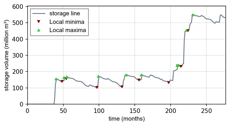
Figure 3:Storage Difference (SD) curve.
Calculate Required Storage Volume
The required storage volume corresponds to the largest difference between a local maximum and its consecutive lowest local minimum. Therefore, add the following lines to the sequent_peak function:
    required_volume = 0.0
    for i, vol in enumerate(list(seas_max_vol):
        try:
            if (vol - seas_min_vol[i]) > required_volume:
                required_volume = vol - seas_min_vol[i]
        except IndexError:
            print("Reached end of storage line.")
Close the sequent_peak function with return required_volume
Call Sequent Peak Algorithm
With all required functions written, the last task is to call the functions in the if __name__ == "__main__" statement:
import ...


def read_data(directory="", fn_prefix="", fn_suffix="", ftype="csv", delimiter=","):
    # see above section


def daily2monthly(daily_flow_series):
    # see above section


def sequent_peak(in_vol_series, out_vol_target):
    # see above descriptions

if __name__ == "__main__":
    # LOAD DATA
    ...
    # CONVERT DAILY TO MONTHLY DATA
    ...
    # MAKE ARRAY OF MONTHLY SUPPLY VOLUMES (IN MILLION CMS)
    monthly_supply = np.array([1.5, 1.5, 1.5, 2.0, 4.0, 4.0, 4.0, 5.0, 5.0, 3.0, 2.0, 1.5])
    # GET REQUIRED STORAGE VOLUME FROM SEQUENT PEAK ALGORITHM
    required_storage = sequent_peak(in_vol_series=monthly_vol_dict, out_vol_target=monthly_supply)
    print("The required storage volume is %0.2f million CMS." % required_storage)
Closing Remarks
The usage of the sequent peak algorithm (also known as Rippl’s method, owing to its original author) has evolved and was implemented in sophisticated storage volume control algorithms with predictor models (statistical and/or numerical).
In the end, there are several algorithms and ways to code them. Many factors (e.g. terrain or climate zone) determine whether seasonal storage is possible or necessary. When determining the storage volume, social and environmental aspects must not be neglected. Every grain of sediment retained is missing in downstream sections of the river, every fish that is no longer able to migrate suffers a loss in habitat, and more than anything else, every inhabitant who suffers economic losses or is even forced to resettle because of the dam must be avoided or adequately compensated.
- Potter, K. W. (1977). Sequent Peak Procedure: Minimum Reservoir Capacity Subject to Constraint on Final Storage. JAWRA Journal of the American Water Resources Association, 13(3), 521–528. 10.1111/j.1752-1688.1977.tb05564.x
- Rippl, W. (1883). The capacity of storage-reservoirs for water-slpply. (including plate). Minutes of the Proceedings of the Institution of Civil Engineers, 71(1883), 270–278. 10.1680/imotp.1883.21797